p2.4 pdf parameterization of boundary layer clouds and turbulence at ...

P2.4

PDF PARAMETERIZATION OF BOUNDARY LAYER CLOUDS AND TURBULENCE AT RESOLUTIONS THAT PERMIT DEEP CONVECTION Vincent E. Larson1∗, , David P. Schanen1 , Minghuai Wang2 , Mikhail Ovchinnikov2 , and Steven Ghan2 1 Dept. of Mathematical Sciences, University of Wisconsin — Milwaukee, Milwaukee, WI 2 Pacific Northwest National Laboratory, Richland, WA

1. INTRODUCTION Convection-permitting simulations have a resolution that permits explicit simulation of deep convection but does not resolve it. Often such simulations have horizontal grid spacings of 2 to 4 km. As computer power has increased in recent years, convection-permitting simulations have become more widely used in practical applications because they avoid the need to use deep convection parameterizations, which are inherently uncertain. Currently, two popular applications of convectionpermitting simulations are 1) climate simulations using a multiscale modeling framework (MMF); and 2) dayahead numerical weather prediction (NWP). MMF simulations embed a cloud-resolving model (CRM) in each column of a general circulation model (GCM) (Khairoutdinov and Randall 2001; Khairoutdinov et al. 2005; Wyant et al. 2006; Khairoutdinov et al. 2008; Tao et al. 2009). The CRMs typically have a horizontal grid spacing of 4 km and therefore permit deep convection. The MMF simulations cited above do prognose subgrid turbulence kinetic energy (TKE) (Tao et al. 2009) or use a Smagorinsky closure for subgrid fluxes, but they do not include parameterizations of sub-CRM cloud fraction or shallow clouds. Because of their coarse vertical and horizontal resolution, standard MMF models may mis-represent low-cloud feedbacks (Blossey et al. 2009). Convection-permitting resolutions are also feasible for NWP forecasts of relatively limited area and short duration. The convection-permitting forecasts of Kain et al. (2008) and Weisman et al. (2008) parameterize subgrid turbulence using the Yonsei University parameterization (Noh et al. 2003), but they do not parameterize subgrid cloud fraction or shallow clouds. However, shallow clouds are important, in part because they are a precursor to deep convection. Unfortunately, although convection-permitting resolutions may permit deep convection, they do not come close to resolving shallow convection, which has important updrafts on the scale of 100 m. This raises the questions: Which aspects of convection-permitting simulations benefit most from a shallow-cloud parameterization? What is the finest horizontal grid spacing at

∗ Corresponding author address: Vincent E. Larson, Department of Mathematical Sciences, University of Wisconsin – Milwaukee, P. O. Box 413, Milwaukee, WI 53201-0413, vlarson at uwm dot edu, http://www.uwm.edu/∼vlarson .

which parameterization of shallow clouds is still beneficial? The answer depends on the type of cloud to be studied and the kind of shallow cloud parameterization used. In this paper, we address these questions by implementing a parameterization of clouds and turbulence in a CRM and testing it for two idealized simulations: one of marine stratocumulus (Sc), and one of trade-wind cumulus (Cu). The parameterization that we will explore is based on the subgrid probability density function (PDF) of vertical velocity, moisture, and heat content (Golaz et al. 2002; Larson and Golaz 2005). It is called “Cloud Layers Unified By Binormals” (CLUBB). For more details on this research, please see the full-length account in Larson et al. (2010).

2. OUR PDF PARAMETERIZATION: CLUBB’S UNDERLYING METHODOLOGY CLUBB is based on the assumed probability density function (PDF) method (Golaz et al. 2002; Larson and Golaz 2005; Larson and Griffin 2010; Griffin and Larson 2010). From the viewpoint of the assumed PDF method, the job of a cloud parameterization is primarily to predict the subgrid joint PDF of vertical velocity, heat content, moisture content, and microphysical quantities. The joint PDF is the probability that the array  vertical velocity, heat content, moisture content, microphysical values  occurs at a particular location and time. PDFs in the atmosphere evolve with time and space, and they contain a wealth of information. Because CLUBB’s PDF includes vertical velocity, we call it a “dynamics-PDF.” The steps in the PDF method may be outlined as follows (e.g. Sommeria and Deardorff 1977; Tompkins 2002). We first write down standard higher-order moment equations based on the equations of fluid flow (Navier-Stokes and advection-diffusion equations). This includes equations for turbulent fluxes and variances of heat and moisture. These equations contain unclosed, higher-order terms. But since we predict the joint PDF of vertical velocity, heat, and moisture, we can close any moments or correlations of these variables. Predicting the full subgrid PDF is computationally infeasible. Therefore we assume a functional form for the PDF, namely a mixture (or sum) of Gaussians. This double Gaussian shape defines a functional form whose width, center, and skewness may vary. Such a form captures well the observed PDF structure in the marine boundary layer (Larson et al. 2001). Within this functional form, we need to determine the particular PDF for each grid box and time step. To do so, we

use the higher-order moments that are prognosed by the model. Once the subgrid PDF is determined, the unclosed moments can be diagnosed directly from the PDF.

3. DESCRIPTION AND CONFIGURATION OF THE CLOUD-RESOLVING MODEL (CRM) The CRM that we use is the System for Atmospheric Modeling (SAM). It is described in Khairoutdinov and Randall (2003). Here we merely note the most salient features. SAM is a non-hydrostatic cloud-resolving model that has been implemented as part of a MMF model (Khairoutdinov et al. 2008) but also can be run at fine resolutions O(10m), that is, as a large-eddy simulation (LES) model. SAM prognoses conservative moisture and heat variables and uses a monotonic flux limiter in order to avoid spurious numerical oscillations. To parameterize subgrid-scale turbulent fluxes, we choose a Smagorinsky option in the code (Khairoutdinov and Randall 2003). Cloud water is diagnosed using saturation adjustment. In order to simulate drizzle, we choose the microphysics scheme of Morrison et al. (2009). In general, the Morrison microphysics is double moment in both rain water and cloud water, but we choose to prescribe cloud droplet number concentration. This choice avoids the complexity of droplet formation processes, and allows us to examine, for prescribed droplet number, how drizzle amount is influenced by the presence of CLUBB’s subgrid parameterizations of moisture and heat content. One difference between convection-permitting NWP forecasts and MMF CRM simulations is that NWP forecasts use a 3D mesh of grid points, whereas MMF simulations typically use a 2D (vertical-horizontal) grid. In this study, we choose to use a 3D grid because it simulates more realistic horizontal winds. We use a stretched grid in the vertical with 128 levels. The grid extends up to 27.5 km and has a grid spacing of ∼ 100 m at 1 km in altitude. We choose this grid because it approximates the resolution that we believe will be used in high-resolution NWP models in the near future. In the horizontal, we use either 2-, 4-, or 16-km grid spacing, which spans the range of grid spacings used in many day-ahead NWP models. The horizontal domain of all simulations is 128 km × 128 km. SAM’s computational timestep is set to 10 s. We will compare simulations in which CLUBB has been implemented in SAM to handle subgrid variability versus those in which CLUBB has not been implemented. When CLUBB is implemented, it is called every 12th SAM timestep in order to save computational expense. Therefore, CLUBB’s timestep is 2 min. When CLUBB is implemented, then for partly cloudy grid boxes, the Morrison microphysics is fed within-cloud averages and the microphysical tendencies are weighted appropriately according to cloud fraction. CLUBB occupies 18% of the total runtime. Finally, we perform a benchmark high-resolution

LES of each case using SAM. Each case is configured according to Gewex Cloud System Study (GCSS) specifications and uses the Morrison microphysics.

4. COMPARISON OF RESULTS WITH AND WITHOUT CLUBB IMPLEMENTED We now discuss results from simulations with and without CLUBB. We analyze a marine stratocumulus case and a shallow cumulus case. Both have been intercompared by GCSS. The first case is a marine Sc layer observed off the coast of California during Research Flight 1 (RF01) of the Second Dynamics and Chemistry of Marine Stratocumulus (DYCOMS-II) field experiment (Stevens et al. 2005). The second case is a trade-wind cumulus layer that is loosely based on observations during the Barbados Oceanographic and Meteorological Experiment (BOMEX) field experiment (Siebesma and Co-authors 2003). In all our plots, thick red lines denote LES benchmark simulations; our goal is to match these fineresolution simulations as closely as possible using coarser-resolution simulations. The dashed lines denote SAM simulations, of various horizontal grid spacings, that do not use CLUBB. The solid lines denote SAM simulations of various grid spacings that do use CLUBB. Our question throughout this section will be: Which matches LES more closely — SAM without CLUBB (dashed lines), or SAM with CLUBB (solid lines)?

4.1

Means and turbulent fluxes of moisture and heat

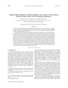
First we present profiles, from both Sc and Cu cases, of horizontally averaged total water mixing ratio (rt ), liquid water potential temperature (θl ), vertical turbulent flux of rt (w rt ), and vertical turbulent flux of θl (w θl ). Fig. 1 shows the RF01 Sc case. With the exception of the SAM standalone profile of rt at 16-km grid spacing, which is not well mixed, all profiles are simulated with satisfactory accuracy. Especially surprising is the remarkably good accuracy of the turbulent fluxes at 16 km, given that those fluxes are grossly underresolved. For the BOMEX trade-wind Cu case (Fig. 2), SAM’s 16-km solution is poor, as expected, with almost no turbulent fluxes above 500 m. SAM’s 4-km solution produces accurate profiles of w θl and θl , but w rt is too small, and consequently rt accumulates near the ground and is not transported upward strongly enough. Overall, SAM simulates rt , θl , w rt , and w θl well at 4-km grid spacing, even though turbulent drafts are severely under-resolved. At 4 km, SAM’s simulated fluxes in the interior are produced mostly by resolved flow rather than the Smagorinsky subgrid parameterization. To achieve this at 4-km grid spacing, SAM simulates a flow field in which the draft width is larger than in

nature but in which the turbulent fluxes have the same magnitude as in LES.

4.2 Variances of w, θl , and rt We now plot and discuss the spatial variances of vertical velocity (w2 ), heat content (θl2 ), and moisture (rt2 ). For the RF01 marine Sc case (Fig. 3), SAM underpredicts w2 moderately at 2-km grid spacing, greatly at 4 km, and severely for 16 km. This is unsurprising, given that simulations at these grid spacings underresolve the drafts. At such grid spacings, generating explicit vertical motion requires overturning an unrealistically wide column of air. Including CLUBB partially mitigates the underprediction and leads to more consistent results at different grid spacings. Although SAM underpredicts w 2 , it overpredicts the scalar variances (i.e. the variances of rt and θl ) at 16and 4-km grid spacings below cloud top. Including CLUBB mitigates the overprediction below cloud top. Both SAM with CLUBB and SAM without CLUBB underpredict a spike in scalar variances at cloud top. In the BOMEX trade-wind Cu case (Fig. 4), SAM again underpredicts w2 , but furthermore, SAM does not produce the bimodal profile of w2 that the LES produces, with one turbulence maximum in the sub-cloud layer, a distinct maximum in the cloud layer, and a minimum within the more stable layer between. Including CLUBB leads to a bimodal w2 profile. Although CLUBB still underpredicts the cloud-layer w2 , it improves the sub-cloud w2 . SAM overpredicts rt2 and θl2 in BOMEX at 2- and 4km grid spacing, but underpredicts them at 16-km grid spacing because that simulation produces little cloud (see Fig. 6 below). When CLUBB is included, the scalar variances for BOMEX are greatly improved at all grid spacings.

4.3

Cloud fraction and cloud water mixing ratio

A primary motivation for including a cloud parameterization in a large-scale model is to better estimate partial cloudiness and cloud water mixing ratio (rc ) in order to calculate their effects on microphysics. We now analyze the quality of the simulations of cloud fraction (cf ) and rc from simulations with and without CLUBB included. First we present cf and rc from the RF01 case (Fig. 5). Except for the 16-km simulation, SAM predicts remarkably accurate profiles of cf and rc . Including CLUBB does not improve the 2- or 4-km RF01 simulations of cf or rc . For the BOMEX trade-wind Cu case (Fig. 6), SAM’s 16-km simulation produces a fog layer because it fails to transport moisture upwards. SAM’s 2- and 4-km simulations predict accurate cf profiles but overpredict rc . Including CLUBB yields a cloud top that is too low but improves the prediction of rc .

4.4

Drizzle

As mentioned above, one motivation for including a cloud parameterization in a large-scale model is to improve the driving of microphysical processes, such as drizzle formation. An accurate microphysics scheme will not produce accurate results if it is fed inaccurate cloud or liquid water fields from a cloud parameterization. In particular, since drizzle processes are often non-linear, accounting for subgrid variability can be important. Fig. 7 presents profiles of drizzle mixing ratio from both cases. With one exception, SAM overpredicts drizzle mixing ratio, sometimes grossly. The exception is the BOMEX case at 16-km grid spacing, which produces no drizzle because it produces little cloud. SAM with CLUBB included also overpredicts drizzle, but not nearly so much. Furthermore, including CLUBB yields much more consistent results with changes in grid spacing. The reason for SAM’s overprediction of drizzle and sensitivity to grid spacing is not clear. However, these problems are probably related to SAM’s overprediction of rt2 and θl2 (Figs. 3–4). Large scalar variances imply pockets of both very moist and very dry air. Drizzle can form readily in the moist pockets, and because of the non-linearity of drizzle processes, the moist pockets can lead to net overprediction of drizzle.

5. CONCLUSIONS In this study, we have implemented a parameterization of clouds and turbulence, CLUBB, into a cloudresolving model, SAM. Then, in order to compare [SAM with CLUBB] to [SAM without CLUBB], we have simulated a marine Sc case (RF01) and a shallow Cu case (BOMEX). The two cases were run at various horizontal grid spacings. Our goal is to address the following two questions: Which aspects of the simulations benefit most from the inclusion of CLUBB? What is the finest horizontal grid spacing at which CLUBB is still beneficial? We find that including CLUBB in SAM has three main benefits: 1) it improves the prediction of variances, both of w and of rt and θl ; 2) it improves the prediction of drizzle mixing ratio; 3) it leads to results that are less sensitive to variations in horizontal grid spacing. We now elaborate on these conclusions. In the following remarks, we do not mean to imply that SAM is inherently defective in any way; all CRMs suffer a degradation in accuracy at coarse resolution. Our goal is merely to inquire about the possible benefits of implementing CLUBB in SAM. First consider the results with 4-km horizontal grid spacing. At 4-km grid spacing, SAM produces accurate simulations of the vertical turbulent flux of rt , w rt , in the RF01 case and the vertical turbulent flux of θl , w θl in both cases. But the inclusion of CLUBB improves, partially at least, the simulation of the horizontally averaged variance of vertical velocity w2 , total wa-

ter mixing ratio rt2 , and liquid water potential temperature θl2 . SAM underpredicts w 2 , as expected, because updrafts and downdrafts are grossly under-resolved at 4-km grid spacing. In contrast, SAM overpredicts r t2 and θl2 . Note that a flux, such as w rt , is closely related to the product of the relevant variances, such as w2 and rt2 . This suggests that SAM predicts w rt accurately through an underprediction in w2 and a compensating overprediction in rt2 . A similar situation holds for θl . Accurate simulation of the variances is important in part because variances drive microphysics. For instance, variations in rt and θl are related to variations in cloud water mixing ratio, rc , and water vapor mixing ratio. These, in turn, influence various processes that form drizzle, such as autoconversion of cloud droplets to form drizzle drops, accretion of cloud droplets onto drizzle drops, and evaporation of drizzle drops below cloud. Perhaps unsurprisingly, then, SAM mispredicts drizzle mixing ratio. In particular, it tends to overpredict drizzle, presumably because SAM produces excessively moist pockets that, through the nonlinearities in autoconversion and accretion, produce excessively large drizzle rates. The inclusion of CLUBB helps ameliorate the problem, but does not entirely remove it, perhaps in part because CLUBB does not account for within-cloud variability of drizzle fields. In the preceding 3 paragraphs, we have discussed results at 4-km horizontal grid spacing. At 16-km grid spacing, SAM produces poor results, as expected, and CLUBB helps mitigate the coarse resolution. This result is unsurprising — 3D models are rarely run at 16-km grid spacing without a cloud parameterization. A less trivial result is that CLUBB helps improve some of the fields even at 2-km grid spacing. CLUBB does not improve the turbulent fluxes at 2 km, but it does improve the shape of the w 2 profile, and, in the cumulus case, it does improve rc , the scalar variances, and drizzle mixing ratio. Finally, we note that the inclusion of CLUBB helps produce results that are more consistent with respect to changes in grid spacing. In most cases, the profiles that include CLUBB are similar except for the 2-km profile, which moves toward the corresponding profile from SAM without CLUBB. This behavior is reasonable. At 2-km grid spacing, more of the motions and variability are resolved, and SAM puts its stamp on the solutions, as desired.

References Blossey, P. N., C. S. Bretherton, and M. C. Wyant, 2009: Subtropical low cloud response to a warmer climate in a superparameterized climate model. Part II. Column modeling with a cloud resolving model. J. Adv. Model. Earth Syst., 1, doi:10.3894/JAMES.2009.1.8. Golaz, J.-C., V. E. Larson, and W. R. Cotton, 2002: A PDF-based model for boundary layer clouds. Part I: Method and model description. J. Atmos. Sci., 59, 3540–3551. Griffin, B. M. and V. E. Larson, 2010: Analytic upscaling of local microphysics parameterizations, Part II: Simulations. Submitted to Quart. J. Royal Met. Soc.. Kain, J. S., D. R. Bright, M. E. Baldwin, J. J. Levit, G. W. Carbin, C. S. Schwartz, M. L. Weisman, K. K. Droegemeier, D. B. Weber, and K. W. Thomas, 2008: Some practical considerations regarding horizontal resolution in the first generation of operational convection-allowing nwp. Wea. Forecasting, 23, 931–952. Khairoutdinov, M. and D. A. Randall, 2001: A cloud resolving model as a cloud parameterization in the NCAR Community Climate System Model: Preliminary results. Geophys. Res. Lett., 28, 3617–3620. Khairoutdinov, M. and D. A. Randall, 2003: Cloud resolving modeling of the ARM Summer 1997 IOP: Model formulation, results, uncertainties, and sensitivities. J. Atmos. Sci., 60, 607–624. Khairoutdinov, M., D. A. Randall, and C. DeMott, 2005: Simulations of the atmospheric general circulation using a cloud-resolving model as a superparameterization of physical processes. J. Atmos. Sci., 62, 2136–2154. Khairoutdinov, M., C. DeMott, and D. A. Randall, 2008: Evaluation of the simulated interannual and subseasonal variability in an amip-style simulation using the csu multiscale modeling framework. J. Climate, 21, 413–431. Larson, V. E. and J.-C. Golaz, 2005: Using probability density functions to derive consistent closure relationships among higher-order moments. Mon. Wea. Rev., 133, 1023–1042.

6. ACKNOWLEDGMENTS

Larson, V. E. and B. M. Griffin, 2010: Analytic upscaling of local microphysics parameterizations, Part I: Theory. Submitted to Quart. J. Royal Met. Soc..

The authors are grateful to NASA for financial support through grant 06-IDS06-0029 and grateful to Dr. Marat Khairoutdinov for the use of his numerical model, SAM.

Larson, V. E., R. Wood, P. R. Field, J.-C. Golaz, T. H. Vonder Haar, and W. R. Cotton, 2001: Small-scale and mesoscale variability of scalars in cloudy boundary layers: One-dimensional probability density functions. J. Atmos. Sci., 58, 1978–1994.

Larson, V. E., D. P. Schanen, M. Wang, M. Ovchinnikov, and S. Ghan, 2010: PDF parameterization of boundary layer clouds in models with horizontal grid spacings from 2 to 16 km. In preparation for Mon. Wea. Rev.. Morrison, H., G. Thompson, and V. Tatarskii, 2009: Impact of cloud microphysics on the development of trailing stratiform precipitation in a simulated squall line: Comparison of one- and two-moment schemes. Mon. Wea. Rev., 137, 993–1009. Noh, Y., W. G. Cheon, S. Y. Hong, and S. Raasch, 2003: Improvement of the K-profile model for the planetary boundary layer based on large eddy simulation data. Bound.-Layer Meteor., 107, 401–427. Siebesma, A. P. and Co-authors, 2003: A large eddy simulation intercomparison study of shallow cumulus convection. J. Atmos. Sci., 60, 1201–1219. Sommeria, G. and J. W. Deardorff, 1977: Subgrid-scale condensation in models of nonprecipitating clouds. J. Atmos. Sci., 34, 344–355. Stevens, B., C.-H. Moeng, A. S. Ackerman, C. S. Bretherton, A. Chlond, S. de Roode, J. Edwards, J.-C. Golaz, H. Jiang, M. Khairoutdinov, M. P. Kirkpatrick, D. C. Lewellen, A. Lock, F. Muller, ¨ D. E. Stevens, E. Whelan, and P. Zhu, 2005: Evaluation of large-eddy simulations via observations of nocturnal marine stratocumulus. Mon. Wea. Rev., 133, 1443– 1462. Tao, W.-K., J. D. Chern, R. Atlas, D. Randall, M. Khairoutdinov, J.-L. Li, D. E. Waliser, A. Hou, X. Lin, C. Peters-Lidard, W. Lau, J. Jiang, and J. Simpson, 2009: A multiscale modeling system: Developments, applications, and critical issues. Bull. Amer. Meteor. Soc., 90, 515–534. Tompkins, A. M., 2002: A prognostic parameterization for the subgrid-scale variability of water vapor and clouds in large-scale models and its use to diagnose cloud cover. J. Atmos. Sci., 59, 1917–1942. Weisman, M. L., C. Davis, W. Wang, K. W. Manning, and J. B. Klemp, 2008: Experiences with 0 to 36-h explicit convective forecasts with the WRF-ARW model. Wea. Forecasting, 23, 407–437. Wyant, M. C., M. Khairoutdinov, and C. S. Bretherton, 2006: Climate sensitivity and cloud response of a GCM with a superparameterization. Geophys. Res. Lett., 33. doi:10.1029/2005GL025464.

Total Water Mixing Ratio, rt

1200

1200

1000

1000

800

800

Height [m]

Height [m]

Liquid Water Potential Temperature,θl

600 3D SAM Standalone 2 km 3D sam 2 km 3D sam_clubb 4 km 3D sam 4 km 3D sam_clubb 16 km 3D sam 16 km 3D sam_clubb

400 200

290

295 300 thetal [K]

600 3D SAM Standalone 2 km 3D sam 2 km 3D sam_clubb 4 km 3D sam 4 km 3D sam_clubb 16 km 3D sam 16 km 3D sam_clubb

400 200

305

2

4

1200

1200

1000

1000

800

800

600 400 200

3D SAM Standalone 2 km 3D sam 2 km 3D sam_clubb 4 km 3D sam 4 km 3D sam_clubb 16 km 3D sam 16 km 3D sam_clubb

−0.04 −0.03 −0.02 −0.01 0 wpthlp / thflux(s) [K m/s]

10

12

Turbulent Flux of rt

Height [m]

Height [m]

Turbulent Flux of θl

6 8 rtm / qt [g/kg]

600 3D SAM Standalone 2 km 3D sam 2 km 3D sam_clubb 4 km 3D sam 4 km 3D sam_clubb 16 km 3D sam 16 km 3D sam_clubb

400 200

0.01

0

1 2 3 4 wprtp / qtflux(s) [(kg/kg) m/s] x 10−5

Figure 1: RF01 profiles averaged over hours 5-6. The panels depict liquid water potential temperature θl (upper left), total water mixing ratio rt (upper right), turbulent flux of θl (lower left), and turbulent flux of rt (lower right). The lines show a benchmark 3D SAM standalone LES (red solid); SAM standalone simulations, with horizontal resolutions of 2 km, 4 km, and 16 km (purple dashed dot, yellow dashed dot, and olive dashed dot, respectively); and SAM simulations that include CLUBB, with horizontal resolutions of 2 km, 4 km, and 16 km (blue solid, gray solid, and green solid lines, respectively). Both SAM with CLUBB and SAM without CLUBB produce adequate simulations of the means and fluxes at 2- and 4-km horizontal grid spacing.

Total Water Mixing Ratio, rt

3000

3000

2500

2500

2000

2000

1500 3D SAM Standalone 2 km 3D sam 2 km 3D sam_clubb 4 km 3D sam 4 km 3D sam_clubb 16 km 3D sam 16 km 3D sam_clubb

1000 500

300

305 thetal [K]

Height [m]

Height [m]

Liquid Water Potential Temperature,θl

3D SAM Standalone 2 km 3D sam 2 km 3D sam_clubb 4 km 3D sam 4 km 3D sam_clubb 16 km 3D sam 16 km 3D sam_clubb

1500 1000 500

310

5

Turbulent Flux of θl 3000 3D SAM Standalone 2 km 3D sam 2 km 3D sam_clubb 4 km 3D sam 4 km 3D sam_clubb 16 km 3D sam 16 km 3D sam_clubb

1500

2000 1500

1000

1000

500

500

−0.03

−0.02 −0.01 0 wpthlp / thflux(s) [K m/s]

3D SAM Standalone 2 km 3D sam 2 km 3D sam_clubb 4 km 3D sam 4 km 3D sam_clubb 16 km 3D sam 16 km 3D sam_clubb

2500

Height [m]

Height [m]

2000

20

Turbulent Flux of rt

3000 2500

10 15 rtm / qt [g/kg]

0

1 2 3 4 5 wprtp / qtflux(s) [(kg/kg) m/s] x 10−5

Figure 2: BOMEX profiles averaged over hours 5-6. The panels depict liquid water potential temperature θl (upper left), total water mixing ratio rt (upper right), turbulent flux of θl (lower left), and turbulent flux of rt (lower right). The lines show a benchmark 3D SAM standalone LES (red solid); SAM standalone simulations, with horizontal resolutions of 2 km, 4 km, and 16 km (purple dashed dot, yellow dashed dot, and olive dashed dot, respectively); and SAM simulations that include CLUBB, with horizontal resolutions of 2 km, 4 km, and 16 km (blue solid, gray solid, and green solid lines, respectively). Both SAM with CLUBB and SAM without CLUBB produce adequate simulations of these fields at 2- and 4-km horizontal grid spacing, except for the flux of rt at 4-km grid spacing.

Variance of w 1200

Variance of w

1000 800

3D SAM Standalone 2 km 3D sam 2 km 3D sam_clubb 4 km 3D sam 4 km 3D sam_clubb 16 km 3D sam 16 km 3D sam_clubb

2500 2000 Height [m]

Height [m]

3000

3D SAM Standalone 2 km 3D sam 2 km 3D sam_clubb 4 km 3D sam 4 km 3D sam_clubb 16 km 3D sam 16 km 3D sam_clubb

600 400

1500 1000

200 500 0

0.1 0.2 wp2 / w2 [m2/s2]

0.3 0

Variance of θl

0.05 0.1 wp2 / w2 [m2/s2]

1200

0.15

Variance of θ

l

3000 1000

3D SAM Standalone 2 km 3D sam 2 km 3D sam_clubb 4 km 3D sam 4 km 3D sam_clubb 16 km 3D sam 16 km 3D sam_clubb

800 Height [m]

Height [m]

2500

600 3D SAM Standalone 2 km 3D sam 2 km 3D sam_clubb 4 km 3D sam 4 km 3D sam_clubb 16 km 3D sam 16 km 3D sam_clubb

400 200

2000 1500 1000 500

0

1

2 2 thlp2 / tl2 [K ]

3

4 0

Variance of r

t

1200

0.1 0.15 0.2 2 thlp2 / tl2 [K ]

0.25

Variance of rt 3D SAM Standalone 2 km 3D sam 2 km 3D sam_clubb 4 km 3D sam 4 km 3D sam_clubb 16 km 3D sam 16 km 3D sam_clubb

1000 800

3000

600 400

3D SAM Standalone 2 km 3D sam 2 km 3D sam_clubb 4 km 3D sam 4 km 3D sam_clubb 16 km 3D sam 16 km 3D sam_clubb

2500

Height [m]

Height [m]

0.05

2000 1500 1000

200 500 0

5 10 15 2 rtp2 / qtp2 [(kg/kg) ]

20 −7

x 10

Figure 3: RF01 profiles averaged over hours 5-6. The panels depict w2 (top), θl2 (middle), and rt2 (bottom). The lines show a benchmark 3D SAM standalone LES (red solid); SAM standalone simulations with horizontal grid spacings of 2 km, 4 km, and 16 km (purple dashed dot, yellow dashed dot, and olive dashed dot, respectively); and SAM simulations that include CLUBB with horizontal grid spacings of 2 km, 4 km, and 16 km (blue solid, gray solid, and green solid lines, respectively).

0

5 10 2 rtp2 / qtp2 [(kg/kg) ]

15 −7

x 10

Figure 4: As in Fig. 3, but for BOMEX profiles averaged over hours 3-6. The panels depict w2 (top), θl2 (middle), and rt2 (bottom). In both RF01 and BOMEX, SAM without CLUBB underpredicts w2 but overpredicts rt2 and θl2 .

CLUBB Cloud Fraction 1200 1000

Cloud Fraction

800

3D SAM Standalone 2 km 3D sam 2 km 3D sam_clubb 4 km 3D sam 4 km 3D sam_clubb 16 km 3D sam 16 km 3D sam_clubb

2500 600 3D SAM Standalone 2 km 3D sam 2 km 3D sam_clubb 4 km 3D sam 4 km 3D sam_clubb 16 km 3D sam 16 km 3D sam_clubb

400 200

2000 Height [m]

Height [m]

3000

1500 1000

0

20

40 60 cld / cld_frac [%]

80

100

500

Cloud Water Mixing Ratio, rc 1200

0

40 60 cld / cld_frac [%]

80

Cloud Water Mixing Ratio, rc 3000

800

3D SAM Standalone 2 km 3D sam 2 km 3D sam_clubb 4 km 3D sam 4 km 3D sam_clubb 16 km 3D sam 16 km 3D sam_clubb

2500

600 3D SAM Standalone 2 km 3D sam 2 km 3D sam_clubb 4 km 3D sam 4 km 3D sam_clubb 16 km 3D sam 16 km 3D sam_clubb

400 200

Height [m]

Height [m]

1000

20

2000 1500 1000

0

1

2 3 rcm / qcl [kg/kg]

4 −4

x 10

Figure 5: RF01 profiles averaged over hours 5-6. The panels depict cloud fraction (top) and liquid water mixing ratio (bottom). The lines show a benchmark 3D SAM standalone LES (red solid); SAM standalone simulations with horizontal resolutions of 2 km, 4 km, and 16 km (purple dashed dot, yellow dashed dot, and olive dashed dot, respectively); and SAM simulations that include CLUBB with horizontal resolutions of 2 km, 4 km, and 16 km (blue solid, gray solid, and green solid lines, respectively). SAM at 2- and 4-km grid spacings produces remarkably accurate profiles of cloud fraction and liquid water.

500

0

5 rcm / qcl [kg/kg]

10 −5

x 10

Figure 6: As in Fig. 5, but for BOMEX profiles averaged over hours 3-6. The addition of CLUBB leads to a more accurate prediction of liquid water for all grid spacings.

Rain Water Mixing Ratio, rr 1200 3D SAM Standalone 2 km 3D sam 2 km 3D sam_clubb 4 km 3D sam 4 km 3D sam_clubb 16 km 3D sam 16 km 3D sam_clubb

Height [m]

1000 800 600 400 200

0

2

4 6 qpl [kg/kg]

8

10 −6

x 10

Rain Water Mixing Ratio, r

r

3000 3D SAM Standalone 2 km 3D sam 2 km 3D sam_clubb 4 km 3D sam 4 km 3D sam_clubb 16 km 3D sam 16 km 3D sam_clubb

Height [m]

2500 2000 1500 1000 500

0

1

2 qpl [kg/kg]

3 −6

x 10

Figure 7: Profiles of drizzle mixing ratio (bottom) from RF01 Sc (upper), and BOMEX trade-wind Cu (lower). Averaging periods are the same as in Figs. (5)–(6). The lines show a benchmark 3D SAM standalone LES (red solid); SAM standalone simulations with horizontal resolutions of 2 km, 4 km, and 16 km (purple dashed dot, yellow dashed dot, and olive dashed dot, respectively); and SAM simulations that include CLUBB with horizontal resolutions of 2 km, 4 km, and 16 km (blue solid, gray solid, and green solid lines, respectively). The addition of CLUBB mitigates the overprediction of drizzle and leads to results that are less sensitive to horizontal grid spacing.