P2.63
IWC AND ICE PRECIPITATION RETRIEVAL ALGORITHMS IN TERMS OF
TEMPERATURE AND RADAR REFLECTIVITY USING OBSERVED ICE SPECTRA Faisal S. Boudala* , George A. Isaac, and David Hudak Cloud Physics and Severe Weather Research Section, Environment Canada, Toronto, Ontario, Canada
1. INTORODUCTION Satellite observations and general circulation model (GCM) studies show that ice clouds have an important impact on earth’s climate by influencing the radiation balance and hydrological cycle (e.g., Ramanathan et al. 1983; Ramaswamy and Ramanathan 1989). However, the value of ice water content (IWC) (e.g., Stephens et al. 2002) and precipitation simulated (e.g., Ebert et al. 2003) using the state of the art numerical models vary significantly. Occasional aircraft in-situ observations provide very useful information about the microphysical properties of clouds, but this data cannot validate climate models on a global scale. Radar technology is increasing being used for remotely retrieving cloud microphysical parameters. Since radar can be operated continuously, it can provide long term measurements of cloud properties. An experimental satellite, CloudSat, that was launched in 2006 (see Stephens et al. 2002), carries a 94 GHz radar. This radar should provide a global picture of cloud microphysical properties including IWC that can be used to constrain these models. However, radar measures the equivalent reflectivity factor ( Ze ) of the cloud particles, but not their mass. The accuracy of the retrieved ice mass or ice precipitation rates based on radar reflectivity is highly dependent on the algorithms used. These algorithms are usually developed based on in-situ aircraft or ground measurements, or in combination with radar and in-situ measurements. In most cases, these retrieval algorithms include just one variable, Ze . Generally, developing a parameterization based on both radar and aircraft in-situ data is not so trivial because of the difference in sampling volume and time lag associated with the two methods (e.g., Hudak et al. 2004). There are several IWC- Ze power law relationships currently used to retrieve IWC, but a modeling study by Sassen and Wang (2002) shows that these power law relationships do not replicate the model calculations. Brown et al. (1995) showed that remotely retrieved IWC using a 94GHz radar can be
___________________________
* Corresponding author address: Faisal S. Boudala Cloud Physics and Severe Weather Research Section, Environment Canada, Toronto, Ontario, Canada, M3H 5T4 E-mail:
[email protected].
accurate within a factor of 2 if Ze alone is used, but this can be improved if the mean size of ice particles is included in the algorithm. Similarly Liu and Illingworth (2002) demonstrated that the inclusion of temperature can improve the accuracy of retrieved IWC. There are several Ze and ice mass flux ( Fm ) relationships (e.g., Zawadzki et al. 1993; Sekhon and Serivastava 1970; Marshall and Palmer 1948). However, they are not adequately validated against observations partly because of the scarcity of surface observation data, especially at high temporal resolution. Nonetheless, the available Ze - Fm relationships do not explicitly include the effects of temperature. Recently, however, such a relationship has been developed (Boudala et al. 2006). In this paper, parameterization of IWC and ice precipitation retrieval algorithms that incorporate Ze and temperature (T) will be presented based on the recent work by Boudala et al. (2006). 2. FIELD MEASUREMENTS The data were collected during several projects using the National Research Council (NRC) Convair580 aircraft. The FIRE Arctic Cloud Experiment (FIRE.ACE) project began in April 1998 and ended in July 1998, with the Convair-580 measurements being made in April (Curry et al. 2000). The First Canadian Freezing Drizzle Experiment (CFDE I) project was conducted in March 1995, and included numerous flights over Newfoundland and the Atlantic Ocean. The Third Canadian Freezing Drizzle (CFDE III) started in December 1997 and ended in February 1998. The first Alliance Icing Research Study (AIRS I) was conducted between 29 November 1999 and 19 February 2000 (Isaac et al. 2001b). The second AIRS (AIRS II) was conducted between November 2003 and February 2004 (Isaac et al. 2005). The Beaufort and Arctic Storms Experiment (BASE) field project was conducted in October 1994 over the Canadian Western Arctic (Gultepe et al. 2000). The data used in this paper is discussed in more details in Boudala et al. (2006). The types of instrumentation used in these projects are described in Isaac et al. (2001a; 2001b; 2005) and Boudala et al. (2006). Nevzorov liquid water content (LWC) and total water content (TWC) probes (Korolev
et al. 1998) which measure LWC and TWC respectively, and the PMS FSSP, 2D-C and 2D-P probes, which measure size, shape and concentration of hydrometers, were used. The temperature was measured with a Rosemount temperature probe. During AIRS II, surface precipitation was measured using the Precipitation Occurrence Sensor System (POSS) that is described by Sheppard (1990). The POSS is X–band low power Doppler radar that measures the terminal velocity and size of cloud particles, as well as their reflectivity. During the AIRS I field project, the McMaster University portable scanning X-band radar was deployed at ground level measuring cloud properties in coordination with aircraft measurements as described by Hudak et al. (2004). The radar scanned the cloud by a series of descending fixed-elevation stares of 90.0, 77.2, 61.5, 49.0, 39.1, 31.1, 24.8, 19.8, 15.0, 12.6 and 10.0 degrees. To match the radar data with the aircraft, the horizontal and vertical distance from the centre of the aircraft sample volume to the centre of the radar resolution cell was determined. In this work, only radar cells within a 1 km horizontal distance from center of aircraft sample volume have been used. The identification of ice clouds follows the Cober et al. (2001) scheme. Based on this scheme, the stratiform ice clouds are characterized by FSSP concentration < 15 cm-3, Rosemount icing detector < 2 mVs-1, and Nevzorov LWC/TWC ratio 0.25 mm 2
,
(1)
where A is the cross-sectional area measured with optical array probes and De is the equivalent melted diameter of an ice particle. Using Eq. (1), the mass of a single ice particle can be given as
m ( A) =
a 3πρ A 3 b 6
,
(2)
where ρ is the density of liquid water. It is most convenient to use equivalent projected cross-sectional area diameter ( D ) of a circle such that A = π D 2 / 4 and transform Eqs. (1) and (2) into a form as m(D) =
0.024 D 2.4 0.1 mm < D ≤ 0.6 mm 0.0334 D 1.86 D > 0.6 mm
,
(3)
where the mass is given in mg and D is given in mm. Note that the exponents in Eq. (3) are similar to coefficients derived based on in-situ observations in midlatitude ice clouds, recently reported by Heymsfield (2003)). This mass-dimensional relationship is give as
m ( D ) = 0.037 D 2.25 ,
(4)
in the same units as Eq. (3). Figure 1a shows a comparison of IWC derived based on Heymsfield (2003) (Eq. 4) and Cunningham (1978) coefficients (Eq. 3) against the IWC measured with the Nevzorov probe. Each point in the figure represents an IWC derived using a 30s averaged ice particle spectra and the small ice particles are added following Boudala et al. (2002). The total data points shown in the figure are about 2036. There is no significant difference between these two schemes as long as D is the same in both cases, and both schemes agree quite well with the observation.
al. (2002a) using a Rayleigh scattering approximation as Z=
6
2
N 0 β 2 Γ(2α + µ + 1)
ρπ
(7)
λ 2α + µ +1
where De is the equivalent melted diameter described earlier. Solving for λ in Eq. (6) and inserting into Eq. (7), IWC can be given in an alternate form following Boudala et al. (2006) as IWC = κ Zγ ,
(8)
where the exponent γ and κ are given as Figure 1a: IWCs measured with Nevzorov probe and derived based using 30s averaged ice spectra measured during CFDE (I and III), FIRE.ACE, and BASE using Heymsfield (2003) and Cunningham (1978) coefficients.
Using the relationships given in Eqs (3) and (4), it is straight forward to derive the mass and radar reflectivity of the measured ice particles, and this will be discussed in the following section. The contribution of small ice particles ( D ≤ 100 µm) are included following Boudala et al. (2002). However, the effect of the small particles on radar reflectivity factor is quite small.
3.2
The Derivation of Radar Reflectivity Factor and IWC
The distribution of ice particles n ( D ) can be represented by a gamma distribution function in a form
n( D) = N 0 D µ exp(−λ D) ,
(5)
where D is the equivalent cross-sectional area diameter of a circle, N 0 is the intercept parameter, µ and λ are the dispersion and slope parameters respectively. Assuming the mass-dimensional relation in a general form as
m(D) = β Dα ,
(6a)
and using Eq. (5), the IWC can be derived following Boudala et al. (2006) as
β N0 IWC = α + µ +1 Γ(α + µ + 1) , λ
(6b)
where Γ is the gamma function. Similarly radar reflectivity can be calculated following Heymsfield et
γ=
α + µ +1 2α + µ + 1
, (9)
κ=
β
( µ +1) − 2α + µ +1
6
ρπ
N0
α 2α + µ +1
Γ(α + µ + 1) γ
2
.
Γ(2α + µ + 1)
As shown in Boudala et al. (2006) if the dispersion (shape) parameter µ is set to zero an exponential distribution function, γ varies from 0.586 to 0.606 corresponding to α = 2.4 and 1.86 respectively, which is very close to 0.6. Actually, this can apply for most of the mass-dimensional relationships where α varies from 1.5 to 3 (Locatelli and Hobbs 1974; Cunningham 1978; Mitchell et al. 1990) resulting in an exponent change only from 0.625 to 0.571 respectively. Since the above expression for κ depends on β -0.21 and β -0.17 depending on which α is used, it is relatively insensitive to the particle habit. However, the dispersion parameter µ could be important in modifying the exponents in the expression given in Eq. (7). Based on midlatitude data, Heymsfield et al. (2002b) showed that the dispersion parameter generally increases with decreasing temperature. For a given mD relationship (see Eq. 3), it is possible to derive µ using the equation provided by Mitchell (1991) as
µ=
(α + 0.67) D − Dm Dm − D
(10)
where Dm is the median mass diameter and D is the mean diameter that can be derived as
Dmax
D=
DN ( D)
Dmin Dmax
.
(11a)
N ( D)
Dmin
3.3 Radar Reflectivity Measurements
Based
On
Aircraft
It is convenient to write Eq. (7) in a form
Both D and Dm can be calculated using ice particle spectra measured with optical array probes. Figure 1b shows D (panel a) and µ (panel b) plotted against temperature as derived based on 2D-C and 2D-P probe measurement data shown in Fig. 1a.
Figure 1b: The mean diameter (a) and dispersion coefficient (b) derived using Eq. 4 and Eq. 10 are plotted against temperature.
Z=
6
ρπ
2 D max
N ( D)m 2 ,
(12)
Dmin
to derive radar reflectivity using aircraft data, where ρ is the density of water and m is given in Eq.(3) or Eq. (4). Figure 2 is taken from Boudala et al. (2006) and shows derived IWC plotted against derived Z based on Eq. (3) using the 30s averaged ice particle size spectra measured with the PMS 2D-C and 2D-P during several field projects. For a given IWC, Z generally increases with increasing temperature. This is consistent with the fact that the mean size of ice particles increases with increasing temperature, which also increases Z . The power law relationships for each temperature interval are also given in the figure. The power law coefficients are increasing with decreasing temperature. For example, γ varies from 0.4 to 0.7 as opposed to just 0.6 as predicted using an exponential function (Eqs. 8 and 9). Figure 3 shows γ calculated using the same data set, but by setting α = 2.4 for the entire spectrum in Eq. (9) since this assumption gave approximately the same IWC as compared to the IWC derived using Eq. (3).
On average, the mean diameter of ice particles increases with increasing temperature as would be expected showing a slight maximum near -12 oC where a maximum in supersaturation with respect to ice is expected. The mean square fit line to the data is given as D = 343.0582 exp(−0.001T 2 − 0.0232T )
(11b)
In contrary to the mean diameter, the dispersion parameter increases with decreasing temperature in agreement with the finding reported by Heymsfield et al. (2002). The mean square fit line in panel b is given as
µ = 5.1456E-4T 2 − 0.0925T − 0.8446
(11c)
Knowing µ and D , it is possible to derive the other coefficients mentioned in Eq. 5 using the relationships given Mitchell (1991).
Figure 2: IWC and Z derived using 30s averaged spectra measured during the CFDE (I and III), FIRE.ACE and BASE projects are plotted for various temperature intervals.
As indicated in the figure, γ increases with decreasing temperature which is consistent with Fig. 2. However, it
is worth mentioning that there is a great deal of scatter in γ , as indicated in Fig. 3, which makes it difficult for the development of an accurate parameterization of an IWC retrieval algorithm using radar reflectivity. However, to a first approximation one can use a linear fit in order to get the approximate value of γ for a given temperature.
IWC = (6.783 x10⁻⁵ T 2 + 0.0262) Z ( −0.0064T + 0.4) ,
(13a)
where T is the temperature in oC and Z is given as mm6 m-3, and IWC is given in gm-3.
4. TESTING THE PARAMETERIZATION The IWC retrieval algorithms currently employed in radar remote sensing application are mainly based on mm wave radar reflectivity measurements, thus they are not directly applicable for Z e determined using the Raleigh scattering approximation. Some of these IWCZ e relationships are summarized in Sassen and Wang (2002). Generally, Z determined based on a Rayleigh approximation is corrected using Mie scattering theory using a formula as
ZMie =
Figure 3: The exponent γ given in Eq. (8) is plotted as a function of temperature.
Inspecting Eq. (9), κ depends on the intercept parameter N 0 and µ . Previous studies by Heymsfield et al. (2002b) and Ryan (2000) showed that N 0 depends on temperature. In order to assess the temperature dependence of κ , the ratio IWC/ Z γ is plotted against temperature in Fig. 4 by setting γ = γ (T) as given in Fig. 3. κ increases with decreasing temperature and this is also consistent with Fig. 2.
(T)
Figure 4: The ratios IWC/ Z derived from 30s averaged ice spectra measured during the CFDE (I and III) , FIRE.ACE and BASE projects are plotted against temperature.
Inspecting Fig. 4, the fitted lines follow a polynomial function of temperature. Therefore, a parameterization is proposed as:
6
ρπ
2 D max
N ( D)m 2 f ( D) ,
(13b)
Dmin
where f ( D) = σ Mie / σ Ray , and the coefficients σ Mie and σ Mie are backscatter cross-sections calculated based on a Rayleigh and Mie scattering model for a given radar frequency respectively. Figure 5a shows the calculated f ( D) for a 94 GHz frequency radar assuming spherical ice and liquid particles at two different temperatures and the corresponding dielectric constants are also given.
Figure 5a: The ratio of calculated back scattered crosssection f ( D ) = σ Mie / σ Ray using Mie and Rayleigh models at 94 GHz are plotted against diameter. Ki and Ki are the dielectric constants for ice spheres (Mätzler (1998) and liquid drops (Liebe et al. 1991).
The Mie backscattering calculation was based on Bohren and Huffman (1983). The dielectric constants are based on Mätzler (1998) for ice and Liebe et al.
(1991) for liquid water. At 94 GHz, the Rayleigh scattering approximation is only valid for D smaller than about 0.6 mm. However, for D greater than 0.6 mm, the Rayleigh scattering approximation significantly overestimates Z . It should be noted that at this radar frequency, the temperature dependence of f ( D) is relatively weak, particularly, for ice particles. Therefore, it is possible to express f ( D) with a simple function as shown in the figure. Using this expression for f ( D) and Eq. 13b, Boudala et al. (2006) derived a relationship between ZMie ( Z94 ) and Z based on the measured ice particle spectra as
Z=1.0681Z941.0612 .
(13c)
The correction factor for low Z values ( Z < 2 mm6 m3 ) appears to be negligible based on this analysis. At Z = 10 mm6 m-3, Z94 is about 18% lower than Z . This power law relationship is found between Z94 and Z can be applied to correct for Z when 94 GHz measurements are being used.
Figure 5b: Various IWC- Z relationships parameterization developed in this work.
and
gives higher IWC as compared to most of the conventional relationships. Therefore, the discrepancy among these relationships may not be explained based on the temperature alone. The new parameterization for temperatures lower than -40 oC were not shown for consistency, since we don’t have in-situ observations for lower temperatures for validation. Figure 6 shows the IWC measured with a Nevzorov probe during the First Alliance Icing Research Study (AIRS I) plotted against the retrieved IWCs based on using the 10 GHz the IWC- Ze relationships McMaster radar data mentioned in Section 2. Also shown are the IWC estimates from the radar data using the parameterization developed in this paper. The results using the conventional IWC- Ze relationships overestimate the ice mass at higher Ze values and underestimate it at lower Ze values, while the parameterization from this paper appear to fit better the one-to-one line. There is considerable scatter for all methods suggesting that the parameterization based on Ze alone appears to be inadequate. However, it should be noted that the accuracy of the direct measurements have some errors, thus more studies are required for further validation of the new parameterization.
the
Figure 5b shows comparisons of the IWC- Ze relationships taken from Sassen and Wang (2002). Since these relationships only involve Ze , it is rather difficult to plot them together with the new parameterizations. However, the parameterizations developed above for temperatures -10 oC, -30 oC, and -40 oC are shown for comparison. Furthermore, Z has to be converted to equivalent radar reflectivity factor ( Ze ) following the convention given in Appendix A (Boudala et al. 2006). At relatively high values of Z , most of the IWC - Z relationships lie within the IWC values calculated using the new parameterization. At low values of Ze , however, the new parameterization
Figure 6: The IWCs retrieved based on observed temperature and Z measured with radar are plotted against the IWC measured with the Nevzorov probe during the AIRS I project.
5.
PRECIPITATION
Using the gamma distribution function discussed earlier and an empirical terminal velocity versus diameter relationship, Boudala et al. (2006) shown that the downward ice mass flux can be given as
ρo Fm = ρa
1/ 2
a 'β N 0Γ(α + µ + b '1) + + λ α + µ + b '1
(14)
a ' and b ' are coefficients associated with terminal velocity ( v = a ' D b '( ρ o / ρ a )1/ 2 see Eq. 18),
where
and the other symbols mean the same as in section 3.1. After substituting the slope parameter from Eq. (6) in into Eq. (14), the downward ice mass flux can be given as
Fm = ΩZ ,
(15)
where the parameters Ω and ω are given as
Ω=
a' β
−(µ +2b '1) + 2α +µ+1
6
ρπ
(b' +α )
N0 2α+µ+1 Γ(α + µ + b '1) + α +µ +b '1 +
2
2α +µ+1
(16)
where D is in mm and v is in m s -1 , ρ 0 = 1 is the reference density, ρ a is the air density. This result also demonstrates the dependence of mass flux on temperature. For a given Fm , increasing temperature increases the reflectivity as a result of the increase in particle size with temperature, which is similar to Fig. 2. The change of ω with temperature in Eq. (17), appears to be mainly due to a change in the dispersion of the ice particle distribution as demonstrated in Fig. 8, which shows ω plotted as a function of temperature. As in the case of Fig. 3, the data shows significant scatter, but the variation in ω with temperature has similar trends as the Z - Fm relations shown in
Fig. 7.
Γ(2α + µ +1)
1
10
-15 oC