P7.2
AN OPERATIONAL METHODOLOGY TO CONTROL RADAR MEASUREMENTS STABILITY FROM MOUNTAIN RETURNS Daniel Sempere-Torres 1, Rafael Sánchez-Diezma 1, M. A Cordoba 1, R . Pascual 2 , Isztar Zawadzki 3 1 Departament d’Enginyeria Hidràulica, Marítima i Ambiental, Universitat Politècnica de Catalunya, Barcelona, Spain. 2 Centre Meteorologic Territorial de Catalunya, Instituto Nacional de Meteorología, Barcelona, Spain 3 J. S. Marshall Radar Observatory, Department of Atmospheric and Oceanic Sciences, McGill University, Montréal, Québec, Canada. 60
1. Introduction
A methodology to monitor and control the stability of radar measurements based on the analysis of the mountain returns is proposed. It has been designed to work operationally on real time, and it is devoted to two objectives: 1) to give a real-time alert in case of large signal instabilities; 2) to estimate a correction factor. 2. Description of the methodology The basis of the proposed methodology is to control radar signal stability through the analysis of temporal variations of ground clutter returns. As reference for the ‘correct’ radar functioning, an average clutter map measured by the volumetrical scanning Cband radar of the Spanish Instituto Nacional de Meteorología (INM) located at Barcelona was determined. M;ain radar characteristics are 0.9° 3-dB beamwidth, λ=5.6 cm, 20 elevation angles. A series of 700 radar maps (i.e approximately 7 day of radar functioning) were selected to calculate the mean map. This data were detailed overviewed to ensure non-precipitating conditions and absence of anomalous propagation. Then for each time step radar stability is analyzed by comparing the ground clutter measured at the first elevation of the present radar image against the average clutter map, which is taken as the correct reference (see Figure 1). The orography of the region covered by the radar is characterized by the increasing altitude of the terrain from the sea to the inner regions. Three major mountain chains can be distinguished. The first two are parallel to the coast, and located inside a strip of terrain at less than 40 km from the sea. These mountains act as a barrier that induces the convection of humid air coming from the sea, favoring the generation and growth of precipitation. The third mountain chain, the Pyrenees, is located at the upper part of the radar coverage (not showed in Figure 1), and exhibits the highest elevations of the region. Figure 1 shows that close to the radar the most intense ground echoes are registered at the second coastal mountain chain. An important area of low terrain-returns, due to the effect of the secondary lobes, is located at the vicinity of the radar and along a strip among the two coastal mountain chains. Corresponding author address: Daniel Sempere -Torres, UPCEHMA, Jordi Girona, 1-3, D1, E-08034 Barcelona. e-mail:
[email protected]
-60 -60
-40
-20
0
20
40
60
distance from the radar (km)
Figure 1. Ground echoes pattern up to 60 km from the radar for the first elevation (0.5°) of the INM radar at Barcelona. A threshold of 23 dBZ was establish in order to determine those values useful for the analysis (i.e. clear interceptions of the main lobe and the terrain). A process of labeling was then applied to the resulting reference map in order to classify all clutter locations. For any available radar image the comparison between reference and present values is performed in the following manner: as a first step all the values of the radar image corresponding to the position of the labeled reference ground clutter are selected. Then a double test is applied in order to reject the ground clutter pre-selected values that: a)
are ‘contaminated’ by the rain (i.e. terraininduced signals are not only due to beam interception but to a joining contribution of rain and ground returns).
b)
suffer from attenuation in the path between ground echoes and radar.
In the first test the average reflectivity around each labeled clutter location is evaluated: a radius of 5 km outward the clutter location is used to define its neighborhood external area. Labeled clutters which neighborhood average reflectivity is > 20 dBZ are discarded from the analysis. The second test rejects echo values that present a reflectivity > Zatt dBZ somewhere along the path from the radar to the echo (presently, we use Zatt = 40 dBZ). Although a method based on the evaluation of the possible degree of attenuation would be more satisfactory we have implement this condition as a first level of complexity. A regression between the valid points is then established in order to compute an over or underdetection factor in dB. This factor, f, is determined as the average deviation of the fitted model respect to the perfect adjustment between 23 dBZ and 40 dBZ. An additional constraint is finally applied in order to assure the robustness of the result, and if the num-
ber of actual valid points, n valid, is smaller that Nmin (Nmin= 30) the resulting correction is rejected. In this case the first previously accepted over sub-detection factor is applyed. As last step a threshold Th = ± 2 dB is applied in order to account for the intrinsic variation of ground echoes in dry conditions (i.e. the correction is applied only if f > 2 dB). This threshold is devised from an analysis of the temporal variation of f under clear air conditions (using the same radar maps employed to define the mean ground clutter map). Figure 2 shows the variation of f along this set of images, where it can be observed a clear long cyclical behavior (each cycle involves a period of approximately 5 hours) between ± 2dB. There is not a clear reason for such a behavior, and the causes are being investigated. Finally, for operational purposes three levels of correction have been established: Robust correction: if nvalid > Nmin , and the correlation between reference and present points is >0.8. d) Not robust correction: if nvalid > Nmin , and the correlation between reference and presentl points is > 0.7 but < 0.8. e) Not possible correction: if nvalid < Nmin , or the correlation between reference and present points is < 0.7. In this case the first previously accepted subdetection factor is used. 2. Case study We have evaluated the performance of the algorithm over different events with severe to light rain over the radar. Figure 3 shows the temporal evolution of the correction factor f, for two studied events, along with different examples of the performance of the algorithm. The different symbols indicate the related level of correction. The first event (June 10, 2000) is characterized by a strong convective activity (first part of the event) followed by a more stratiform period. c)
In the first images of the event a long squall line moves from south to east inside the radar coverage area and the algorithm provides ‘no correction is necessary’ result (f > 2 dB). The scatterplot 1 in Figure 3 shows an example of this period. The comparison between reference and present ground clutter is plotted using crosses for the valid values (not attenuated, and not rain contaminated) and dots for the rest of the points. Notice that most of the dots are clearly located out of the 1:1 line, underestimating the clutter intensities (attenuated values) or overestimating them (i.e. it rains over the clutter). From image 16 to 20 the radar itself and its vicinity was affected by the squall line, so that a general attenuation is observed (see scatterplot 2). The resulting valid points don’t allow the algorithm to define a robust correction factor, and their clear dispersion could be related to the fact that the methodology used to discard the attenuated values is not effective in this case. After image 20 the correction is more stable, indicating an under-detection greater then 5 dB. Scatter-
plot 3 in Figure 3 shows an example of this period: most of the valid points are regularly shifted above the line 1:1. This under-detection over such period could be due to a temporal radar failure or the remnant effect of the previous rain over the radome. The second temporal evolution of f correspond with a more light convective event (20 October 2000). The most interesting feature of this event is the performance of the correction in cases of anomalous propagation (AP) in dry weather (as in the first 5 images of the event). Scatterplot 4 in Figure 3 shows an example of this situation. The AP effect increases the dispersion of the comparison, which is reasonable since ground echo locations for the observed values does not correspond with the mean ones. The result is a overdetection factor, which could be used as an indicator of this type of problems, although its application could not be easy in case of rain. 4. Conclusions The proposed stability algorithm aims to be a primary tool to monitor and control the radar signal. Along the studied events it has deserved a reasonable performance except for intense rain over the radar (general attenuation). Future development should be done in order to improve the detection of attenuation among the radar and the ground clutter, using an improved algorithm able to compute the path integrated attenuation. On the other hand it would be necessary to study the effectiveness of the algorithm as a function of the size of the ground echoes included in the analysis, its distance from the radar or their related degree of beam interception. This study could provide which are the most suitable terrain-induced echoes for the optimum performance of the proposed algorithm. 4. Acknowledgements: This work has been done in the frame of the R+D CICYT project REN2000-17755-C01. Thanks are due to the Spanish Instituto Nacional de Meteorología for providing radar data and support. 5. References Della-Bruna, G., J. Joss, and R. Lee, Automatic calibration and verification of radar accuracy for precipitation estimation, in 27th Conference On Radar Meteorology, edited by AMS, Vail, Colorado, USA, 1997. Delrieu, G., J.D. Creutin, and H. Andrieu, Simulation of radar mountain returns using a digitized terrain model, J. Atmos. Oceanic Technol., 12, 1038-1049, 1995. Delrieu, G., L. Hucke, and J.D. Creutin, Attenuation in rain for X- and C-band weather radar systems: sensitivity with respect to the drop size distribution., J. Appl. Meteorol., 38, 57-68, 1999. Manz, A., J. Handwerker, M. Löffler-Mang, R. Hannesen, and H. Gysi, Radome influence on weather radar systems with emphasis to rain effects, in 29th Conference On Radar Meteorology, edited by AMS, pp. 918-921, Montreal, Quebec, Canada, 1999
correction factor (dB)
10 5 0 -5 -10 0
200
400 image index
600
Figure 2. Temporal evolution of the f factor in dry weather conditions.
correction factor (dB)
15
2
3
10
1
5 0 -5 0
20
40
60
80
100
120
correction factor (dB)
image index 10 8
4
6 4 2 0 -2 -4 0
100
200 image index Not possible correction Not robust correction
1
2
number of valid points = 327 correction factor = -0.28 r 2 = 0.94
60
40
20
number of valid points = 124 correction factor = 13.14 r 2= 0.23
60
40
0 0
80
20
40 60 present (dBZ)
80
0
4
number of valid points = 342 correction factor = 7.07 2 r = 0.83
60
reference (dBZ)
reference (dBZ)
80
20
0
3
400
Robust correction Correction not necessary
reference (dBZ)
reference (dBZ)
80
300
40
20
80
20
40 60 presentl (dBZ)
80
number of valid points = 595 correction factor = -3.53 r 2= 0.64
60
40
20
0
0 0
20
40 60 present (dBZ)
80
0
20
40 60 present (dBZ)
80
Figure 3. Above: temporal evolution of the f factor along two analyzed event. The symbols indicate the robustness of the f calculation. The four scatterplots below show different examples comparing the ground clutters from a given radar image against the values on the reference mean map.