PAC-Bayesian Compression Bounds on the Prediction ... - CiteSeerX

PAC-Bayesian Compression Bounds on the Prediction Error of Learning Algorithms for Classification Thore Graepel ([email protected]) Institute of Computational Science, ETH Z¨ urich, Switzerland

Ralf Herbrich ([email protected]) Microsoft Research, 7 J J Thomson Avenue, CB3 0FB Cambridge, UK

John Shawe-Taylor ([email protected]) Department of Computer Science, Royal Holloway, University of London, UK Abstract. We consider bounds on the prediction error of classification algorithms based on sample compression. We refine the notion of a compression scheme to distinguish permutation and repetition invariant and non-permutation and repetition invariant compression schemes leading to different prediction error bounds. Also, we extend known results on compression to the case of non-zero empirical risk. We provide bounds on the prediction error of classifiers returned by mistakedriven online learning algorithms by interpreting mistake bounds as bounds on the size of the respective compression scheme of the algorithm. This leads to a bound on the prediction error of perceptron solutions that depends on the margin a support vector machine would achieve on the same training sample. Furthermore, using the property of compression we derive bounds on the average prediction error of kernel classifiers in the PAC-Bayesian framework. These bounds assume a prior measure over the expansion coefficients in the data-dependent kernel expansion and bound the average prediction error uniformly over subsets of the space of expansion coefficients.

1. Introduction Generalization error bounds based on sample compression are a great example of the intimate relationship between information theory and learning theory. The general relation between compression and prediction has been expressed in different contexts such as Kolmogorov complexity (Vit`anyi and Li, 1997), minimum description length (Rissanen, 1978), and information theory (Wyner et al., 1992). As was first pointed out by Littlestone and Warmuth (1986) and later by Floyd and Warmuth (1995), the prediction error of a classifier h can be bounded in terms of the number d of examples to which a training sample of size m can be compressed while still preserving the information necessary for the learning algorithm to identify the classifier h. Intuitively speaking, the remaining m − d examples that are not required for training serve as a test sample on which the classifier is evaluated. Interestingly, the c 2004 Kluwer Academic Publishers. Printed in the Netherlands. °

revision.tex; 3/11/2004; 21:59; p.1

2 compression bounds so derived are among the best bounds in existence in the sense that they return low values even for moderately large training sample size. As a consequence, compression arguments have been put forward as a justification for a number of learning algorithms including the support vector machine (Cortes and Vapnik, 1995) whose solution can be reproduced based on the support vectors, that constitute a subset of the training sample. Prediction error bounds based on compression stand in contrast to classical PAC/VC bounds in the sense that PAC/VC bounds assume the existence of a fixed hypothesis space H (see Cannon et al. (2002) for a relaxation of this assumption) while compression results are independent of this assumption and typically work well for algorithms based on a hypothesis space of infinite VC dimension or even based on a data-dependent hypothesis space, as is the case, for example, in the support vector machine. We systematically review the notion of compression as introduced in Littlestone and Warmuth (1986) and Floyd and Warmuth (1995). In Section 3 we refine the idea of a compression scheme to distinguish between permutation and repetition invariant and non permutation and repetition invariant compression schemes, leading to different prediction error bounds. Moreover, we extend the known compression results for the zero-error training case to the case of non-zero training error. Note that the results of both Littlestone and Warmuth (1986) and Floyd and Warmuth (1995) implicitly contained this agnostic bound via the notion of side information. We then review the relation between batch and online learning, which has been a recurrent theme in learning theory (see Littlestone (1989) and Cesa-Bianchi et al. (2002)). The results in Section 4 are based on an interesting relation between online learning and compression: Mistake-driven online learning algorithm constitute non permutation invariant compression schemes. We exploit this fact to obtain PAC type bounds on the prediction error of classifiers resulting from mistake-driven online learning using mistake bounds as bounds on the size d of compression schemes. In particular, we will reconsider the perceptron algorithm and derive a PAC bound for the resulting classifiers from a mistake bound involving the margin a support vector machine would achieve on the same training data. This result went so far largely unnoticed in the study of margin bounds. Similarly to PAC/VC results, recent bounds in the PAC-Bayesian framework (Shawe-Taylor and Williamson, 1997; McAllester, 1998) assume the existence of a fixed hypothesis space H. Given a prior measure PH over H the PAC-Bayesian framework then provides bounds on the average prediction error of classifiers drawn from a posterior PH|Z=z in terms of the average training error and the KL divergence between prior

revision.tex; 3/11/2004; 21:59; p.2

3 and posterior (McAllester, 1999). Interestingly, tight margin bounds for linear classifiers were proved in the PAC-Bayesian framework in Graepel et al. (2000), Herbrich and Graepel (2002) and Langford and Shawe-Taylor (2003). Heavily borrowing from ideas in the compression framework, in Section 5 we prove general PAC-Bayesian results for the case of sparse data-dependent hypothesis spaces such as the class of kernel classifiers on which the support vector machine is based. Instead of assuming a prior PH over hypothesis space, we assume a prior PA over the space of coefficients in the kernel expansion. As a result, we obtain PAC-Bayesian results on the average prediction error of data-dependent hypotheses.

2. Basic Learning Task and Notation We consider the problem of binary classification learning, that is, we aim at modeling the underlying dependency between two sets referred to as input space X and output space Y, which will be jointly referred to as the input-output space Z according to the following definition: Definition 1 (Input-Output space). We call 1. X the input space, 2. Y := {−1, +1} the output space, and 3. Z := X × Y the joint input-output space of the binary classification learning problem. Learning is based on a training sample z of size m defined as follows: Definition 2 (Training sample). Given an input-output space Z and a probability measure PZ thereon we call an m-tuple z ∈ Z m drawn IID from PZ := PXY a training sample of size m. Given z = ((x1 , y1 ) , . . . , (xm , ym )) we will call the pairs (xi , yi ) training examples. Also we use the notation x = (x1 , . . . , xm ) and similarly y = (y1 , . . . , ym ). The hypotheses considered in learning are contained in the hypothesis space. Definition 3 (Hypothesis and hypothesis space). Given an input space X and an output space Y we define a hypothesis as a function h:X →Y,

revision.tex; 3/11/2004; 21:59; p.3

4 and a hypothesis space as a subset H ⊆ YX . A hypothesis space is called a data-dependent hypothesis space if the set of hypotheses can only be defined for a given training sample and may change with varying training samples. A learning algorithm takes a training sample and returns a hypothesis according to the following definition: Definition 4 (Learning algorithm). Given an input space X and an output space Y we call a mapping1 A : Z (∞) → Y X a learning algorithm. In order to assess the quality of solutions to the learning problem, we use the zero-one loss function. Definition 5 (Loss function). Given an output space Y we call a function l : Y × Y → R+ a loss function on Y and we define the zero-one loss function as ½

l0−1 (ˆ y , y) :=

0 for yˆ = y . 1 for yˆ 6= y

Note that this can also be written as l0−1 (ˆ y , y) = Iyˆ6=y , where I is the indicator function. A useful measure of success of a given hypothesis h based on a given loss function l is its (true) risk defined as follows: Definition 6 (True risk). Given a loss function l, a hypothesis space H, and a probability measure PZ the functional R : H → R given by R [h] := EXY [l (h (X) , Y)] , that is, the expectation of the loss, is called the (true) risk on H. Given a hypothesis h we also call R [h] its prediction error. For the zero-one loss l0−1 the risk is equal to the probability of error. The true risk or its average over a subset of hypotheses will be our main quantity of interest. A useful estimator for the true risk is its plug-in estimator, the empirical risk. 1

Throughout the paper we use the shorthand notation A(i) := ∪ij=1 Aj .

revision.tex; 3/11/2004; 21:59; p.4

5 Definition 7 (Empirical risk). Given a training sample z ∼ PZm , a loss function l : Y × Y → R, and an hypothesis h ∈ H we call |z|

X ˆ [h, z] := 1 R l (h (xi ) , yi ) |z| i=1

ˆ [h, z] = 0 is called the empirical risk of h on z. An hypothesis h with R consistent with z. Given these preliminaries we are now in a position to consider bounds on the true risk of classifiers based on the property of sample compression. 3. PAC Compression Bounds In order to relate our new results to the body of existing work, we will review the unpublished work of Littlestone and Warmuth (1986) and the seminal paper Floyd and Warmuth (1995). In addition to these two papers, our introduction of compression schemes carefully distinguishes between permutation and repetition invariance since it leads to different bounds on the prediction error. This distinction will become important when studying online algorithms in Section 4. 3.1. Compression and Reconstruction In order to be able to bound the prediction error of classifiers in terms of their sample compression it is necessary to consider particular learning algorithms instead of particular hypothesis spaces. In contrast to classical results that constitute bounds on the prediction error which hold uniformly over all hypotheses in H (PAC/VC framework) or which hold uniformly over all subsets of H (PAC-Bayesian framework) we are in the following concerned with bounds on the prediction error which hold only for those classifiers that result from particular learning algorithms (see Definition 4). Let us decompose a learning algorithm A into a compression scheme as follows (Littlestone and Warmuth, 1986). Theorem 1 (Compression scheme). We define the set Id,m ⊂ {1, . . . , m}d as the set containing all index vectors of size d ∈ N, n

o

Id,m := (i1 , . . . , id ) ∈ {1, . . . , m}d . Given a training sample z ∈ Z m and an index vector i ∈ Id,m let z i be the subsequence indexed by i, z i := (zi1 , . . . , zid ) .

revision.tex; 3/11/2004; 21:59; p.5

6

x2

1

−1 −1

1 x

1

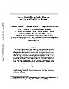
Figure 1. Illustration of the convergence of the kernel classifier based on class-conditional Parzen window density estimation to the nearest neighbor classifier in X = [−1, +1]2 ⊂ R2 . For σ = 5 the decision surface (thin line) is almost linear, for σ = 0.4 the curved line (medium line) results, and for very small σ = 0.02 the piecewise linear decision surface (thick line) of nearest neighbor results. For nearest neighbor only the circled points contribute to the decision surface and form the compression sample.

We call an algorithm A : Z (∞) → H a compression scheme ifSand only S m if there exists a pair (C, R) of functions C : Z (∞) → ∞ m=1 d=1 Id,m (compression function) and R : Z (∞) → H (reconstruction function) such that we have for all training samples z, ³

´

A (z) = R z C(z) . We call the compression scheme permutation and repetition invariant if and only if the reconstruction function R is invariant under permutation and repetition of training examples in any training sample z. The quantity |C (z)| is called the size of the compression scheme. The definition of a compression scheme is easily illustrated by three well-known algorithms: the perceptron, the support vector machine (SVM), and the K-nearest-neighbors (KNN) classifier, which are all based on the data-dependent hypothesis space of kernel classifiers.

revision.tex; 3/11/2004; 21:59; p.6

7 Definition 8 (Kernel classifiers). Given a training sample z ∈ (X × Y)m and a kernel function k : X × X → R we define the datadependent hypothesis Hk (x) by (

Hk (x) :=

x 7→ sign

Ãm X i=1

!¯ ) ¯ ¯ m . αi k (xi , x) ¯ α ∈ R ¯

(1)

1. The (kernel) perceptron algorithm (Rosenblatt, 1962) is a compression scheme that is not permutation and repetition invariant. Rerunning the perceptron algorithm on a training sample that consists only of those training examples that caused an update in the previous run leads to the same classifier as before. Permuting the order of the examples or omitting repeated examples, however, may lead to a different classifier. 2. The support vector machine (Cortes and Vapnik, 1995) is a permutation and repetition invariant compression scheme. Rerunning the SVM only on the support vectors leads to the same classifier regardless of their order because the expansion coefficients in the optimal solution of the other training examples are zero and the objective function is invariant under permutation of the training examples. 3. The K-nearest-neighbors classifier (Cover and Hart, 1967) can be viewed as a limiting case of kernel classifiers and can be viewed as a permutation and repetition invariant compression scheme as well: Delete those training examples that do not change the majority on any conceivable test input x ∈ X (consider Figure 3.1 for an illustration for the case of K = 1). Note that mere sparsity in the expansion coefficients αi in (1) is not sufficient for an algorithm to qualify as a compression scheme, but it is necessary that the hypothesis found can be reconstructed from the compression sample. The relevance vector machine algorithm presented in Tipping (2001) is an example of an algorithm that does provide solutions that are sparse in the expansion coefficients αi without constituting a compression scheme. Based on the concept of compression let us consider PAC-style bounds on the prediction error of learning algorithms as described above.

revision.tex; 3/11/2004; 21:59; p.7

8 3.2. The Realizable Case Let us first consider the realizable learning scenario, i.e. for every trainˆ [h, z] = 0. Then ing sample z there exists a classifier h such that R we have the following compression bound (note that (2) was already proven in Littlestone and Warmuth (1986) but will be repeated here for comparison). Theorem 2 (PAC compression bound). Let A : Z (∞) → H be a compression scheme. For any probability measure PZ , any m ∈ N, and any δ ∈ (0, 1], with probability at least 1 − δ over the random draw of ˆ [A (z) , z] = 0 and d := |C (z)| then the training sample z ∈ Z m , if R µ

R [A (z)] ≤

µ ¶¶

³ ´ 1 1 log md + log (m) + log m−d δ

,

and, if A is a permutation and repetition invariant compression scheme, then Ã

à !

µ ¶!

m 1 1 log + log (m) + log R [A (z)] ≤ m−d d δ

.

(2)

Proof. First we bound the probability ³

´

ˆ [A (Z) , Z] = 0 ∧ R [A (Z)] > ε ∧ |C (Z)| = d PZm R ³

³

´´

ˆ [R (Zi ) , Z] = 0 ∧ R [R (Zi )] > ε ≤ PZm ∃i ∈ Id,m : R ≤

X

³

´

ˆ [R (Zi ) , Z] = 0 ∧ R [R (Zi )] > ε . PZm R

(3)

i∈Id,m

³

´

The second line follows from the property A (z) = R z C(z) and the fact that the event in the second line is implied by the event of the first line. The third line follows from the union bound, Lemma 1 in Appendix A. Each summand in (3)—being a product measure—is further bounded by h

³

´i

ˆ [R (z i ) , Z] = 0 ∧ R [R (z i )] > ε EZd PZm−d |Zd =zi R

(4)

where we used the fact that correct classification of the whole training ˜ ⊆ z of it. Since sample z implies correct classification of any subset z the m − d remaining training examples are drawn IID from PZ we can apply the binomial tail bound, Theorem 7 in Appendix A, thus bounding the probability in (4) by exp (− (m − d) ε). The number of different index vectors i ∈ Id,m is given by md = |Id,m ¡ |¢for the case that R is not permutation and repetition invariant and m d in the case that

revision.tex; 3/11/2004; 21:59; p.8

9 R is permutation and repetition invariant. As a result, the probability ¡ ¢ in (3) is strictly less than md exp (− (m − d) ε) or m exp (− (m − d) ε), d respectively. We have with probability at least 1 − δ over the random draw of the training sample z ∈ Z m that the proposition Υd (z, δ) defined by ³

ˆ [A (z) , z] = 0 ∧ |C (z)| = d ⇒ R [A (z)] ≤ R

´

log md + log

³ ´ 1 δ

m−d

¡m¢

md

holds true (with replaced by d for the permutation and repetition invariant case). Finally, we apply the stratification lemma, Lemma 1 in 1 Appendix A, to the sequence of propositions Υd with PD (d) = m for all d ∈ {1, . . . , m}. The bound (2) in Theorem 2 is easily interpreted if we consider the ¡ ¢ ¡ em ¢d bound on the binomial coefficient, m , thus obtaining2 d < d µ

R [A (z)] ≤

µ

2 em d log m d

¶

µ ¶¶

1 δ

+ log (m) + log

.

(5)

This result should be compared to the simple VC bound (see, e.g., Cristianini and Shawe-Taylor (2000)), µ

µ

2 2em ε (m, dVC , δ) = dVC log2 m dVC

¶

µ ¶¶

+ log2

2 δ

.

(6)

Ignoring constants that are worse in the VC bound, these two bounds almost look alike. The (data-dependent) number d of examples needed by the compression scheme replaces the VC dimension dVC := VCdim (H) of the underlying hypothesis space. Compression bounds can thus provide bounds on the prediction error of classifiers even if the classifier is chosen from an hypothesis space H of infinite VC dimension. The relation between VC bounds and compression schemes—motivated by equations such as (5) and (6)—is still not fully explored (see Floyd and Warmuth (1995) and recently Warmuth (2003)). We observe an interesting analogy between the ghost sample argument in VC theory (see Herbrich (2001) for an overview) and the use of the remaining m−d examples from the sample. While the uniform convergence requirement in VC theory forces us to assume an extra ghost sample to be able to bound the true risk, the m−d training examples serve the same purpose in the compression framework: To measure an empirical risk that serves to bound the true risk. The second interesting observation about Theorem 2 is that the bound for a permutation and repetition invariant compression scheme 2

Note that the bound is trivially true for d >

m ; 2

otherwise

1 m−d

≤

2 . m

revision.tex; 3/11/2004; 21:59; p.9

10 is slightly better than its counterpart without this invariance. This difference can be understood from a coding point of view: It requires more bits to encode a sequence of indices (where order and repetition matter) as compared to a set of indices (where order does not matter and there are no repetitions). In the proof of the PAC compression bound, Theorem 2, the stratification over the number d of training examples used was carried out 1 using a uniform (prior) measure PD (1) = · · · = PD (m) = m indicating complete ignorance about the sparseness to be expected. In a PACBayesian spirit, however, we may choose a more “natural” prior that expresses our prior belief about the sparseness to be achieved. To this end we assume that given a training sample z ∈ Z m the probability p that any given example zi ∈ z will be in the compression sample z C(z) is constant and independent of z. This induces a distribution over d = |C (z)| given for all d ∈ {1, . . . , m} by à !

PD (d) =

m d p (1 − p)m−d , d

P

for which we have m i=1 PD (i) ≤ 1 as required for the stratification lemma, Lemma 1 in Appendix A. The value p thus serves as an a-priori d belief about the value of the observed compression coefficient pˆ := m . This alternative sequence leads to the following bound for permutation and repetition invariant compression schemes, µ

µ ¶

1 R [A (z)] ≤ 2 · pˆ log p

µ

1 + (1 − pˆ) log 1−p

³ ´

³

¶

µ ¶¶

1 1 + log m δ

. (7)

´

1 Note that the term pˆ log p1 + (1 − pˆ) log 1−p can be interpreted as the cross entropy between two random variables that are Bernoullidistributed with success probabilities p and pˆ, respectively. For an illustration of how a suitably chosen value p of the expected compression ratio can decrease the bound value for a given value pˆ of the compression ratio consider Figure 3.2.

3.3. The Unrealizable Case The previous compression bound indicates an interesting relation between PAC/VC theory and data compression. Of course, data compression schemes come in two flavors, lossy and non-lossy. Thus it comes as no surprise that we can derive bounds on the prediction error of compression schemes also for the unrealisable case with non-zero empirical risk (Graepel et al., 2000). Note that these results are implicitly contained in Floyd and Warmuth (1995) where the authors consider the

revision.tex; 3/11/2004; 21:59; p.10

0.3 0.2

d/m=0.005 d/m=0.01 d/m=0.02 d/m=0.04

0.0

0.1

Bound on Prediction Error

0.4

0.5

11

0.00

0.02

0.04

0.06

0.08

0.10

Expected Compression Ratio

Figure 2. Dependency of the PAC-Bayesian compression bound (7) on the expected value p and the observed value pˆ of the compression coefficient. For increasing values d the optimal choice of the expected compression ratio p increases as indicated pˆ := m by the shifted minima of the family of curves (m = 1000, δ = 0.05).

more general scenario that the reconstruction function R also gets r bits of side-information. Theorem 3 (Lossy compression bound). Let A : Z (m∞) → H be a compression scheme. For any probability measure PZ , any m ∈ N, and any δ ∈ (0, 1], with probability at least 1 − δ over the random draw of the training sample z ∈ Z m , if d = |C (z)| the prediction error of A (z) is bounded from above by R [A (z)] ≤

m ˆ R [A (z) , z] + m−d

v ³ ´ u u log (md ) + 2 log (m) + log 1 t δ

2 (m − d)

,

and, if A is a permutation and repetition invariant compression scheme, then by

R [A (z)] ≤

m ˆ R [A (z) , z] + m−d

v ³ ´ u ¡ ¢ u log m + 2 log (m) + log 1 t δ d

2 (m − d)

.

revision.tex; 3/11/2004; 21:59; p.11

12 Proof. Fixing the number of training errors q ∈ {1, . . . , m} and |C (z)| we bound—in analogy to the proof of Theorem 2—the probability µ

¶

ˆ [A (Z) , Z] ≤ q ∧ R [A (Z)] > ε ∧ |C (Z)| = d PZm R m µ ¶ X ˆ [R (Zi ) , Z] ≤ q ∧ R [R (Zi )] > ε . (8) ≤ PZm R m i∈I d,m

ˆ [A (z) , z] ≤ q implies (m − d) · R ˆ [A (z) , z¯] ≤ q for We have that m · R i ¯ all i ∈ Im,d and i := {1, . . . , m} \ i leading to an upper bound, ·

µ

EZd PZm−d |Zd =zi

¶¸

ˆ [R (z i ) , Z] ≤ R

q ∧ R [R (z i )] > ε m−d

, (9)

on the probability in (8). From Hoeffding’s inequality, Theorem 8 in Appendix A, we know for a given sample z i that the probability in (9) is bounded by Ã

µ

q exp −2 (m − d) ε − m−d

¶2 !

.

d The number of different index vectors i ∈ Id,m is again given by m ¡m¢for the case that R is not permutation and repetition invariant and d in the case that R is permutation and repetition invariant. Thus we have with probability at least 1 − δ over the random draw of the training sample z ∈ Z m for all compression schemes A and maximal number of training errors q that the proposition Υd,q (z, δ) given by

ˆ [A (z) , z] ≤ R

q m

∧ |C (z)| = d

⇒r log(md )+log( 1δ ) q R [A (z)] ≤ m−d + 2(m−d) ¡ ¢

holds true (with md replaced by m d for the permutation invariant case). Finally, we apply the stratification lemma, Lemma 1 in Appendix A, to the sequence of propositions Υd,q with PDQ ((d, q)) = m−2 for all (d, q) ∈ {1, . . . , m}2 . The above theorem is proved using a simple combination of Hoeffding’s inequality and a double stratification about the number d of non-zero coefficients and the number of empirical errors, q. From an information theoretic point of view the first term of the right hand side of the inequalities represents the number of bits required to explicitly

revision.tex; 3/11/2004; 21:59; p.12

13 transfer the labels of the misclassified examples—this establishes the link to the more general results of Floyd and Warmuth (1995). Note also that Marchand and Shawe-Taylor (2001) prove a similar result to Theorem 3, avoiding the square root in the bound at the cost of a less straight-forward argument and worse constants.

4. PAC Bounds for Online Learning In this section we will review the relation between PAC bounds and mistake bounds for online learning algorithms. This relation has been studied before and Theorem 4 is a direct consequence of Theorem 3 in Floyd and Warmuth (1995). In light of the relationship, we will reconsider the perceptron algorithm and derive a PAC bound for the resulting classifiers from a mistake bound involving the margin a support vector machine would achieve on the same training data. We will argue that a large potential margin is sufficient to obtain good bounds on the prediction error of all the classifiers found by the perceptron on permuted training sequences z j . Although this result is a straightforward application of Theorem 4 it went unnoticed and is, so far, missing in any comparative study of margin bounds—which form the theoretical basis of all margin based algorithms including the support vector machine algorithm. 4.1. Online-Learning and Mistake Bounds In order to be able to discuss the perceptron convergence theorem and the relation between mistake bounds and PAC bounds in more depth let us introduce formally the notion of an online algorithm (Littlestone, 1988). Definition 9 (Online learning algorithm). Consider an update function U : Z × H → H and an initial hypothesis h0 ∈ H. An online S (∞) learning algorithm is a function A : Z (∞) × ∞ × m=1 {1, . . . , m} m H → H that takes a training sample z ∈ Z , a training sequence j ∈ S∞ (∞) , and an initial hypothesis h0 ∈ H, and produces m=1 {1, . . . , m} the final hypothesis AU (z) := h|j| of the |j|-fold recursion of the update function U, hi := U (zji , hi−1 ) . Mistake-driven learning algorithms are a particular class of online algorithms that only change their current hypothesis if it causes an error on the current training example.

revision.tex; 3/11/2004; 21:59; p.13

14 Definition 10 (Mistake-driven learning algorithm). An online algorithm AU is called mistake-driven if the update function satisfies for all x ∈ X , for all y ∈ Y, and for all h ∈ H that y = h (x)

⇒

U ((x, y) , h) = h .

In the PAC framework we focus on the error of the final hypothesis A (z) an algorithm produces after considering the whole training sample z. In the analysis of online-algorithms one takes a slightly different view: The number of updates until convergence is considered the quantity of interest. Definition 11 (Mistake bound). Consider an hypothesis space H, a training sample z ∈ Z m labeled by a hypothesis h ∈ H and a sequence j ∈ {1, . . . , m}(∞) . Denote by ˜j ⊆ j the sequence of mistakes, i.e., the subsequence of j containing the indices ji ∈ {1, . . . , m} for which hi−1 6= hi . We call a function MU : Z (∞) → N a mistake bound for the online algorithm AU if it bounds the number |˜j| of mistakes AU makes on z ∈ Z m , |˜j| ≤ MU , for any ordering j ∈ {1, . . . , m}(∞) . In a sense, this is a very practical measure of error assuming that a learning machine is learning “on the job”. 4.2. From Online to Batch Learning Interestingly, we can relate any mistake bound for a mistake-driven algorithm to a PAC style bound on the prediction error: Theorem 4 (Mistake bound to PAC bound). Consider a mistakedriven online learning algorithm AU for H with a mistake bound MU : Z (∞) → N. For any probability measure PZ , any m ∈ N, and any δ ∈ (0, 1], with probability at least 1 − δ over the random draw of the training sample z ∈ Z m we have that the true risk R [AU (z)] of the hypothesis AU (z) is bounded from above by µ

µ ¶¶

2 1 R [AU (z)] ≤ (MU (z) + 1) log (m) + log m δ

.

(10)

Proof. The proof is based on the fact that a mistake-driven algorithm constitutes a (non permutation and repetition invariant) compression scheme. Assume we run AU twice on the same training sample z and training sequence j. From the first run we obtain the sequence of mistakes ˜j. Thus we have for the compression function C, C (z j ) := ˜j .

revision.tex; 3/11/2004; 21:59; p.14

15 Running AU only on z˜j then leads to the same hypothesis as before, ³

´

AU (z, j) = AU z, ˜j

showing that the reconstruction function R is given by the algorithm AU itself. The compression scheme is in general not permutation and repetition invariant because AU and hence R is not. We can thus apply 1 2 Theorem 2, where we bound d from above by MU and use m−d ≤ m m for all d ≤ 2 . Let us consider two examples for the application of this theorem. The first example illustrates the relation between PAC/VC theory and the mistake bound framework: Example 1 (Halving algorithm). For finite hypothesis spaces H, |H| < ∞, the so-called halving algorithm A1/2 (Littlestone, 1988) achieves a minimal mistake bound of M1/2 (z) = dlog2 (|H|)e . The algorithm proceeds as follows: 1. Initialize the set V0 := H and t = 0. 2. For a given input xi ∈ X predict the class yˆi ∈ Y that receives the majority of votes from classifiers h ∈ Vt , yˆi = argmax |{h ∈ Vt : h (xi ) = y}| . y∈Y

3. If a mistake occurs, that is yi 6= yˆi , all classifiers h ∈ Vt that are inconsistent with xi are removed, Vt+1 := Vt \ {h ∈ Vt : h (xi ) 6= yi } . 4. If no more mistakes occur, return any classifier h ∈ Vt ; otherwise goto 2. Plugging the value M1/2 (z) into the bound (10) gives h

i

R A1/2 (z) ≤

µ

µ ¶¶

2 1 (dlog2 (|H|)e + 1) log (m) + log m δ

,

which holds uniformly over version space VM and up to a factor of 2 log (m) recovers what is known as the cardinality bound in PAC/VC theory.

revision.tex; 3/11/2004; 21:59; p.15

16 The second example provides a surprising way of proving bounds for linear classifiers based on the well-known margin γ by a combination of mistake bounds and compression bounds: Example 2 (Perceptron algorithm). The perceptron algorithm Aperc is possibly the best-known mistake-driven online algorithm (Rosenblatt, 1962). The perceptron convergence theorem provides a mistake bound for the perceptron algorithm given by µ

Mperc (z) =

ς (x) γ ∗ (z)

¶2

,

with ς 2 (x) := maxxi ∈x kxi k being the data radius3 and γ ∗ (z) := max min yi hxi , wi / kwk , w

(xi ,yi )∈z

being the maximum margin that can be achieved on z. Plugging the value Mperc (z) into the bound (10) gives 2 R [Aperc (z)] ≤ m

Ãõ

ς (x) γ ∗ (z)

¶2

!

µ ¶!

+ 1 log (m) + log

1 δ

.

This result bounds the prediction error of any solution found by the perceptron algorithm in terms of the quantity ς (x) /γ ∗ (z), that is, in terms of the margin γ ∗ (z) a support vector machine (SVM) would achieve on the same data sample z. Remarkably, the above bound gives lower values than typical margin bounds (Vapnik, 1998; Bartlett and Shawe-Taylor, 1998; Shawe-Taylor et al., 1998) for classifiers w in terms of their individual margins γ (w, z) that have been put forward as justifications of large margin algorithms. As a consequence, whenever the SVM appears to be theoretically justified by a large observed margin γ ∗ (z), every solution found by the perceptron algorithm has a small guaranteed prediction error—mostly bounded more tightly than current bounds on the prediction error of SVMs.

5. PAC-Bayesian Compression Bounds In the proofs of the compression results, Theorem 2 and Theorem 3, we made use of the fact that m − d of the m training examples had not been used for constructing the classifier and could thus be used to bound the true risk with high probability. In this section, we will make 3

Note that in this example we assume xi ∈ RN and w ∈ RN .

revision.tex; 3/11/2004; 21:59; p.16

17 use of similar arguments in order to deal with data-dependent hypothesis spaces such as those parameterized by α in kernel classifiers. This function class constitutes the basis of support vector machines, Bayes point machines, and other kernel classifiers (see Herbrich (2001) for an overview). Note that our results neither rely on the kernel function k to be positive definite or even symmetric nor is is relevant which algorithm is used to construct the final kernel classifiers. For example, these bounds also apply to kernel classifiers learned with the relevance vector machine. Obviously, typical VC results cannot be applied to this type of data-dependent hypothesis class, because the hypothesis class is not fixed in advance. Hence, its complexity cannot be determined before learning4 . In this section we will proceed similarly to McAllester (1998): First we prove a PAC-Bayesian “folk” theorem, then we proceed with a PAC-Bayesian subset bound. 5.1. The PAC-Bayesian Folk Theorem for Data-Dependent Hypotheses Suppose instead of a PAC-Bayesian prior PH over a fixed hypothesis space we define a prior PA over the sequence α of expansion coefficients αi in (1). Relying on a sparse representation with kαk0 < m we can then prove the following theorem: Theorem 5 (PAC-Bayesian bound for single data-dependent classifiers). For any prior probability distribution PA on a countable subset A ⊂ Rm satisfying PA (α) > 0 for all α ∈ A, for any probability measure PZ , any m ∈ N, and for all δ ∈ (0, 1] we have with probability at least 1 − δ over the random draw of the training sample zh ∈ Z mi that for any hypothesis h( ,x) ∈ Hk (x) the prediction error R h( ,x) is bounded by h

R h(

µ

i ,x)

≤

µ

1 1 log m − kαk0 PA (α)

¶

µ ¶¶

+ log

1 δ

.

Proof. First we show that the proposition Υ (z, kαk0 , δ), 

h

i

h

i

ˆ h( ,x) , z = 0 ⇒ R h( ,x) ≤ Υ (z, kαk0 , δ) := R

log

³ ´  1 δ

m − kαk0

,

(11) 4 A fixed hypothesis space is a pre-requisite in the VC analysis because it appeals to the union bound over all hypotheses which are distinguishable by their predictions on a double sample (see Herbrich (2001) for more details).

revision.tex; 3/11/2004; 21:59; p.17

18 holds for all α ∈ A with probability at least 1−δ over the random draw of z ∈ Z m . Let i ∈ Id,m , d := kαk0 , be the index vector with entries at which αi 6= 0. Then we have for all α ∈ A that ³

h

ˆ h( PZm R

i

h

i

,X) , Z = 0 ∧ R h(

³

h

ˆ h( ≤ PZm R h

,Xi ) , Z

³

< (1 − ε)

h

= 0 ∧ R h( h

ˆ h( ≤ EZd PZm−d |Zd =zi R m−d

,X)

i

´

>ε i

i

,Xi )

´

>ε

h

,xi ) , Z = 0 ∧ R h(

i ,xi )

´i

>ε

≤ exp (−ε (m − d)) .

The key is that the classifier h( ,x) does not change over the random draw of the m − d examples not used in its expansion. Finally, apply the stratification lemma, Lemma 1 in Appendix A, to the proposition Υ (z, kαk0 , δ) with PA (α). Obviously, replacing the binomial tail bound with Hoeffding’s inequality, Theorem 8, allows us to derive a result for the unrealisable case with non-zero empirical risk. This bound then reads h

i

R h(

,x)

h

≤

m ˆ h( R m − kαk0

i ,x)

+

v ´ ³ ¡m¢ u 1 u log t PA ( ) + log δ

2 (m − kαk0 )

.

Remark 1. Note that both these results are not direct consequences of Theorem 2 and 3 since in these new results the bound depends on both the sparsity kαk0 and the prior PA (α) of the particular hypothesis h( ,x) as opposed to only the sparsity d of the compression scheme that produced h in Theorem 2 and 3. Note that any prior PA over a finite subset of nα’s is effectively encoding oa prior over infinitely many hypotheses h( ,x) |x ∈ X m , PA (α) > 0 . It is not possible to incorporate such a prior into both Theorem 2 or 3 using the union bound. Example 3 (1-norm soft margin perceptron). Suppose we run the (kernel) perceptron algorithm with box-constraints 0 ≤ αi ≤ C (see, e.g., Herbrich (2001)) and obtain a classifier h( ,x) with d non-zero coefficients αi . For a prior PA (α) :=

1

¡ ¢ m k mk (2C + 1)k k0

(12)

0

over the set {α ∈ h

R h(

i ,x)

≤

Rm | α

m ˆh R h( m−d

∈ {−C, . . . , 0, . . . , C}m } we get the bound i ,x)

+

v ³ ´ u ¡ ¢ u log m + d log (2C + 1) + log m2 t δ d

2 (m − d)

,

revision.tex; 3/11/2004; 21:59; p.18

19 which yields lower values than the compression bound, Theorem 3, for non-permutation and repetition invariant compression schemes if (2C + 1) < d. This can be seen by bounding log (d!) by d log (d) in Theorem 3 using Stirling’s formula, Theorem 10 in Appendix A. 5.2. The PAC-Bayesian Subset Bound for Data-Dependent Hypotheses Let us now consider a PAC-Bayesian subset bound for the data-dependent hypothesis space of kernel classifiers (1). In order to make the result more digestible we consider it for a fixed number d of non-zero coefficients. Theorem 6 (PAC-Bayesian bound for subsets of data-dependent classifiers). For any prior probability distribution PA , for any probability measure PZ , for any m ∈ N, for any d ∈ {1, . . . , m}, and for all δ ∈ (0, 1] we have with probability at least 1 − δ over the random draw of the training sample z ∈ Z m that for any subset A, PA (A) > 0, with constant sparsity d and zero empirical risk, ∀α ∈ Ah : hkαk0 ii = h i ˆ d ∧ R h( ,x) (z) = 0, the average prediction error EA|A∈A R h(A,x) is bounded by h

h

³

ii

EA|A∈A R h(A,x)

≤

log

1 PA (A)

³ ´

´

1 δ

+ 2 log (m) + log

+1

m−d

.

Proof. Using the fact that the loss function l0−1 is bounded from above by 1, we decompose the expectation at some point ε ∈ R by h

h

ii

EA|A∈A R h(A,x) ³

h

≤

i

´

³

h

i

´

ε · PA|A∈A R h(A,x) ≤ ε + 1 · PA|A∈A R h(A,x) > ε . (13) As in the proof of Theorem 5 we have that for all α ∈ A and for all δ ∈ (0, 1], PZm |A= (Υ (Z, d, δ)) ≥ 1 − δ , where the proposition Υ (z, d, δ) is given by (11). By the quantifier reversal lemma, Lemma 2 in Appendix A, this implies that for all β ∈ (0, 1) with probability at least 1−δ over the random draw of the training sample z ∈ Z m for all γ ∈ (0, 1], ³ ³

h

³

1

PA|Zm =z ¬ΥA z, d, (γβδ) 1−β i

h

i

´´ ´

ˆ h(A,x) , z = 0 ∧ R h(A,x) > ε (γ, β) PA|Zm =z R

< γ < γ

revision.tex; 3/11/2004; 21:59; p.19

20 with

³

ε (γ, β) :=

log

1 δγβ

´

(1 − β) (m − d)

.

Since the distribution over α is by assumption a prior and thus independent of the data, we have PA|Zm =z = PA and hence h

h

i

³

i

PA|A∈A R h(A,x) > ε (γ, β) =

h

ˆ h( because by assumption α ∈ A implies R γ=

and β = h

1 m

h

µ

≤ ε (γ, β) · 1 − ³

= Exploiting that

1 m

≤

i ,x) , z

= 0. Now choosing

we obtain from (13)

ii

EA|A∈A R h(A,x)

´

PA (A)

γ ≤ , PA (A)

PA (A) m

i

h

PA A ∈ A ∧ R h(A,x) > ε (γ, β)

1 m−d

log

1 PA (A)

´

γ PA (A)

¶

+

γ PA (A)

+ 2 log (m) + log m−d

³ ´ 1 δ

+

1 . m

completes the proof.

Again, replacing the binomial tail bound with Hoeffding’s inequality, Theorem 8, allows us to derive a result for the unrealisable case with non-zero empirical risk. Example 4 (1-norm soft margin permutational perceptron sampling). Continuing the discussion of Example 3 with the same prior distribution (12) consider the following procedure: Learn a 1-norm soft margin perceptron with box constraints 0 ≤ αi ≤ C for all i ∈ {1, . . . , m} and assume linear separability. Permute the compression sample z isv and retrain to obtain an ensemble A := {α1 , . . . , αN } of N different coefficient vectors αj . Then the PAC-Bayesian subset bound for data dependent hypotheses, Theorem n 6, bounds theoaverage prediction error of the ensemble of classifiers h( ,x) | α ∈ A corresponding to the ensemble A of coefficient vectors.

6. Conclusions We derived various bounds on the prediction error of sparse classifiers based on the idea of sample compression. Essentially, the results rely on

revision.tex; 3/11/2004; 21:59; p.20

21 the fact that a classifier h( ,x) resulting from a compression scheme (of size d) is independent of the random draw of m − d training examples, which—if classified with low or zero empirical risk by h( ,x) —serve to ensure a low prediction error with high probability. Our results in Section 4 relied on an interpretation of mistake-driven online learning algorithms as compression schemes. The mistake bound was then used as an upper bound on the size of the compression sample and thus lead to bounds on the prediction error of the final hypothesis returned by the algorithm. This procedure emphasizes the conceptual difference between our results and typical PAC/VC results: PAC/VC theory makes statements about uniform convergence within particular hypothesis classes H. In contrast, compression results rely on assumptions about particular learning algorithms A. This idea (which is carried further in Herbrich and Williamson (2002)) is promising in that it leads to bounds on the prediction error that are closer to the observed values and that take into account the actual learning algorithm used. We extended the PAC-Bayesian results of McAllester (1998) to datadependent hypotheses that are represented as linear expansions in terms of training inputs. The theorems are thus applicable to the class of kernel classifiers as defined in Definition 8, ranging from support vector to K-nearest-neighbors classifiers. Empirically, the bounds given yield rather low bound values and have low constants in comparison to VC bounds or bounds based on the observed margin. In summary, they are widely applicable and rather tight. The formulation of a prior over expansion coefficients α that parameterize data-dependent hypotheses appears rather unusual. No contradiction, however, arises because the prior cannot be used to “cheat” by adjusting it in such a way as to manipulate the bound values. The reason is that the expansion (1) does not contain the labels yi . Instead the prior serves to incorporate a-priori knowledge about the representation of classifiers in terms of training inputs. Of course, there exist many non-sparse classifiers with a low prediction error as well. It remains a challenging open question how we can formulate and prove PAC-Bayesian bounds for data-dependent hypotheses that are dense, i.e., that have few or no non-zero coefficients. Note that the PAC-Bayesian results in Langford and Shawe-Taylor (2003) only apply to a fixed hypothesis space by the assumption of a positive definite and symmetric kernel ensuring a fixed feature space.

revision.tex; 3/11/2004; 21:59; p.21

22 Appendix A. Basic Results As a service to the reader we provide some basic results in the appendix for reference. Proofs using a rigorous and unified notation consistent with this paper can be found in Herbrich (2001). A.1. Tail Bounds At several points we require bounds on the probability mass in the tails of distributions. Assuming the zero-one loss, the simplest such bound is the binomial tail bound. Theorem 7 (Binomial tail bound). Let X1 , . . . , Xn be independent random variables distributed Bernoulli (µ). Then we have that PXn

à n X

!

Xi = 0 = (1 − µ)n ≤ exp (−nµ) .

i=1

For the case of non-zero empirical risk, we use Hoeffding’s inequality (Hoeffding, 1963) that bounds the deviation between mean and expectation for bounded IID random variables. Theorem 8 (Hoeffding’s inequality). Given n independent bounded random variables X1 , . . . , Xn such that for all i PXi (Xi ∈ [a, b]) = 1, then we have for all ε > 0 Ã

PXn

!

n 1X Xi − EX [X] > ε n i=1

Ã

2nε2 < exp − (b − a)2

!

.

A.2. Binomial Coefficient and Factorial For bounding combinatorial quantities the following two results are useful. Theorem 9 (Bound on binomial coefficient). For all m, d ∈ N with m ≥ d we have à !

m log d

µ

em ≤ d log d

¶

Theorem 10 (Simple Stirling’s approximation). For all n ∈ N we have n (log (n) − 1) < log (n!) < n log (n)

revision.tex; 3/11/2004; 21:59; p.22

23 A.3. Stratification In order to be able to make probabilistic statements uniformly over a given set we use a generalization of the so-called union bound, which we refer to as the stratification or multiple testing lemma. Lemma 1 (Stratification). Suppose we are given a set {Υ1 , . . . , Υs } of s measurable logic formulae Υ : Z (m) × (0, 1] → {true, false} and a discrete probability measure PI over the sample space {1, . . . , s}. Let us assume that ∀i ∈ {1, . . . , s} : ∀m ∈ N : ∀δ ∈ (0, 1] :

PZm (Υi (Z, δ)) ≥ 1 − δ .

Then, for all m ∈ N and δ ∈ (0, 1], PZm

às ^

!

Υi (Z, δPI (1)) ≥ 1 − δ .

i=1

A.4. Quantifier Reversal The quantifier reversal lemma is an important building block for some PAC-Bayesian theorems (McAllester, 1998). Lemma 2 (Quantifier reversal). Let X and Y be random variables with associated probability spaces (X , X, PX ) and (Y, Y, PY ), respectively, and let δ ∈ (0, 1]. Let Υ : X × Y × (0, 1] → {true, false} be any measurable formula such that for any x and y we have {δ ∈ (0, 1] | Υ (x, y, δ) } = (0, δmax ] for some δmax ∈ (0, 1]. If ∀x ∈ X : ∀δ ∈ (0, 1] : PY|X=x (Υ (x, Y, δ)) ≥ 1 − δ , then for any β ∈ (0, 1) we have ∀δ ∈ (0, 1] that ³

³

³

1

PY ∀α ∈ (0, 1] : PX|Y=y Υ X, y, (αβδ) 1−β

´´

´

≥ 1−α ≥ 1−δ.

References Bartlett, P. and J. Shawe-Taylor: 1998, ‘Generalization Performance of Support Vector Machines and other Pattern Classifiers’. In: Advances in Kernel Methods — Support Vector Learning. MIT Press, pp. 43–54.

revision.tex; 3/11/2004; 21:59; p.23

24 Cannon, A., J. M. Ettinger, D. Hush, and C. Scovel: 2002, ‘Machine Learning with Data Dependent Hypothesis Classes’. Journal of Machine Learning Research 2, 335–358. Cesa-Bianchi, N., A. Conconi, and C. Gentile: 2002, ‘On the generalization ability of on-line learning algorithms’. In: Advances in Neural Information Processing Systems 14. Cambridge, MA, MIT Press. Cortes, C. and V. Vapnik: 1995, ‘Support Vector Networks’. Machine Learning 20, 273–297. Cover, T. M. and P. E. Hart: 1967, ‘Nearest neighbor pattern classifications’. IEEE Transactions on Information Theory 13(1), 21–27. Cristianini, N. and J. Shawe-Taylor: 2000, An Introduction to Support Vector Machines. Cambridge, UK: Cambridge University Press. Floyd, S. and M. Warmuth: 1995, ‘Sample Compression, learnability, and the Vapnik Chervonenkis dimension’. Machine Learning 27, 1–36. Graepel, T., R. Herbrich, and J. Shawe-Taylor: 2000, ‘Generalisation error bounds for sparse linear classifiers’. In: Proceedings of the Annual Conference on Computational Learning Theory. pp. 298–303. Herbrich, R.: 2001, Learning Kernel Classifiers: Theory and Algorithms. MIT Press. Herbrich, R. and T. Graepel: 2002, ‘A PAC-Bayesian margin bound for linear classifiers’. submitted to IEEE Transactions on Information Theory. Herbrich, R. and R. C. Williamson: 2002, ‘Algorithmic Luckiness’. Journal of Machine Learning Research 3, 175–212. Hoeffding, W.: 1963, ‘Probability Inequalities for Sums of Bounded Random Variables’. Journal of the American Statistical Association 58, 13–30. Langford, J. and J. Shawe-Taylor: 2003, ‘PAC-Bayes and Margins’. In: Advances in Neural Information Processing Systems 15. Cambridge, MA, pp. 439–446, MIT Press. Littlestone, N.: 1988, ‘Learning Quickly When Irrelevant Attributes Abound: A New Linear-treshold Algorithm’. Machine Learning 2, 285–318. Littlestone, N.: 1989, ‘From on-line to batch learning’. In: Proceedings of the second Annual Conference on Computational Learning Theory. pp. 269–284. Littlestone, N. and M. Warmuth: 1986, ‘Relating Data Compression and Learnability’. Technical report, University of California Santa Cruz. Marchand, M. and J. Shawe-Taylor: 2001, ‘Learning with the Set Covering Machine’. In: Proceedings of the Eighteenth International Conference on Machine Learning (ICML’2001). San Francisco CA, pp. 345–352, Morgan Kaufmann. McAllester, D. A.: 1998, ‘Some PAC Bayesian Theorems’. In: Proceedings of the Annual Conference on Computational Learning Theory. Madison, Wisconsin, pp. 230–234, ACM Press. McAllester, D. A.: 1999, ‘PAC-Bayesian Model Averaging’. In: Proceedings of the Annual Conference on Computational Learning Theory. Santa Cruz, USA, pp. 164–170. Rissanen, J.: 1978, ‘Modeling by Shortest Data Description’. Automatica 14, 465– 471. Rosenblatt, F.: 1962, Principles of Neurodynamics: Perceptron and Theory of Brain Mechanisms. Washington D.C.: Spartan–Books. Shawe-Taylor, J., P. L. Bartlett, R. C. Williamson, and M. Anthony: 1998, ‘Structural Risk Minimization over Data-Dependent Hierarchies’. IEEE Transactions on Information Theory 44(5), 1926–1940.

revision.tex; 3/11/2004; 21:59; p.24

25 Shawe-Taylor, J. and R. C. Williamson: 1997, ‘A PAC Analysis of a Bayesian Estimator’. Technical report, Royal Holloway, University of London. NC2–TR– 1997–013. Tipping, M.: 2001, ‘Sparse Bayesian Learning and the Relevance Vector Machine’. Journal of Machine Learning Research 1, 211–244. Vapnik, V.: 1998, Statistical Learning Theory. New York: John Wiley and Sons. Vit` anyi, P. and M. Li: 1997, ‘On Prediction by Data Compression’. In: Proceedings of the European Conference on Machine Learning. pp. 14–30. Warmuth, M.: 2003, ‘Open Problems: Compressing to VC Dimension Many Points’. In: Proceedings of the Annual Conference on Computational Learning Theory. Wyner, A. D., J. Ziv, and A. J. Wyner: 1992, ‘On the role of pattern matching in information theory’. IEEE Transactions on Information Theory 4(6), 415–447.

revision.tex; 3/11/2004; 21:59; p.25