Prediction and Trace Compression of Data Access Addresses through Nested Loop Recognition A. Ketterlin
Ph. Clauss
Département d’Informatique Université Louis Pasteur Strasbourg (France)
ICPS/LSIIT (CNRS, UMR 7005) Université Louis Pasteur Strasbourg (France)
[email protected]
[email protected]
ABSTRACT This paper describes an algorithm that takes a trace (i.e., a sequence of numbers or vectors of numbers) as input, and from that produces a sequence of loop nests that, when run, produces exactly the original sequence. The input format is suitable for any kind of program execution trace, and the output conforms to standard models of loop nests. The first, most obvious, use of such an algorithm is for program behavior modeling for any measured quantity (memory accesses, number of cache misses, etc.). Finding loops amounts to detecting periodic behavior and provides an explanatory model. The second application is trace compression, i.e., storing the loop nests instead of the original trace. Decompression consists of running the loops, which is easy and fast. A third application is value prediction. Since the algorithm forms loops while reading input, it is able to extrapolate the loop under construction to predict further incoming values. Throughout the paper, we provide examples that explain our algorithms. Moreover, we evaluate trace compression and value prediction on a subset of the SPEC2000 benchmarks.
Categories and Subject Descriptors D.4.8 [Operating Systems]: Performance—Modeling and prediction
General Terms Performance, Algorithms
Keywords Trace analysis, nested loop recognition, data access, trace compression, value prediction
1.
INTRODUCTION
Memory behavior is an important factor to consider when attempting to optimize the performance of a program. One
Permission to make digital or hard copies of all or part of this work for personal or classroom use is granted without fee provided that copies are not made or distributed for profit or commercial advantage and that copies bear this notice and the full citation on the first page. To copy otherwise, to republish, to post on servers or to redistribute to lists, requires prior specific permission and/or a fee. CGO’08, April 5–10, 2008, Boston, Massachusetts, USA. Copyright 2008 ACM 978-1-59593-978-4/08/0004 ...$5.00.
way to record such behavior is to use traces from the execution of the program. Traces of the instructions executed, as well as memory locations accessed by the program are both useful for optimization. Data accesses however, can reveal many opportunities for optimizing for the memory hierarchy of a system. Data access traces though can be extremely large, making the storage and the analysis of such data a challenge. A wide range of compression techniques have been proposed in prior work [2, 4, 5, 7, 8, 9, 11]. These approaches significantly reduce the size of traces, but unfortunately do not employ a codec format that is human-readable or easy to analyze directly. Many of these approaches for data access encode access strides and the number of repeated instances of these strides as a way of facilitating compression and/or prediction of future access patterns. However, such approaches are limited to encoding linear access patterns and do not capture relationships between or across such patterns. In this paper, we propose to represent address traces as sequences of loop nests whose loop bounds and innermost level instructions are linear functions of the loop indices. When calculated, these functions result in the address values of the compressed trace. This representation enables us to compress data address traces with a compression rate that outperforms the best-performing approaches for trace compression and prediction. Moreover, our encoding method captures (and makes available for direct analysis) repetitions, hierarchical and linear relationships, stride values, and access patterns. Our algorithm for generating this representation is fast, incremental and can be applied using one single pass. We achieve decompression by executing directly the loop nest program that our compression algorithm produces. Furthermore, we are able to combine our approach with other, general purpose compression algorithms such as bzip2. We have evaluated our compression utility on data access traces using a subset of the SPEC CPU2000 benchmarks, that we execute on an Itanium-2 system. In addition to compression, our algorithm can be used as an on-line predictor of future data access behavior. After a short learning phase, we use the detected loop nests to predict the next referenced addresses, by artificially extending some loop bounds. Since the representation format is a program, it can be dynamically compiled in the context of a dynamic optimizer. We have evaluated our prediction mechanism for several scenarios using the SPEC2000 loop nest programs that our compression utility generates.
The paper is organized as follows. Section 2 details the loop recognition process: it explains the loop detection and formation techniques, details the structure of loop nests, and describes an efficient algorithm. Section 3 presents a straightforward application of loop nest recognition to trace compression. The algorithm is evaluated in terms of its compression ratio, and compared to some of the best known compression algorithms. Section 4 describes the use of loop nest recognition for value prediction. Using the algorithm’s internal structures provides a means to predict future values, up to an arbitrary distance. The paper concludes with some remarks on the algorithm, and presents some plans for further development.
2.
EXTRACTING LOOPS FROM EXECUTION TRACES
The problem we face consists in determining one or more loop nests such that, when executed, these loop nests exactly produce a given sequence of numbers. We describe an algorithm that solves this problem. This section starts with a description of the basic operations that lie at the core of the method, then proceeds to provide a formal description of the loop nests that are produced, and finally explicits an algorithm that can efficiently produce loop nests from sequences of numbers. Some remarks on obvious extensions to the structure of loop nests, on the overall computational complexity of the process, and on relevant prior work known to the authors conclude the section.
2.1
Detecting loops in traces
The basic idea of the algorithm consists, in its simplest incarnation, in detecting linear progressions in a sequence of numbers. For example, it is immediate to detect that the sequence 3, 10, 17, 24, 31 is an arithmetic progression because the stride between successive values is constant. Several trace compression techniques have used this fact to compress (slices of) traces into a triple consisting of the initial value, the increment and the overall number of elements. Because the present work focuses on actually producing loops, this sequence will be explicitly written as: for i = 0 to 4 val 3 + 7i When run, this loop produces the initial sequence. Suppose now that new values appears, e.g., 38 and 45. It is obvious again that the loop can be “extended” to cover these values: every subsequent value that “conforms” to the body of the loop for the next values of the loop index can be integrated by a simple increment of the loop’s upper bound. The first subsequent value that breaks the progression can be used as a potential start for a new loop, and the process continues, leading to a sequence of numbers and simple loops. The algorithm presented below is based on the exact same principle, except that it is able to turn several successive loops into new, deeper loops, so as to construct loop nests as complex as necessary to cover the input sequence. The loop nest building procedure relies on two simple operations. The first operation recognizes the start of a loop and forms its initial syntactic structure. The second operation recognizes that what follows a loop is just a new iteration of the loop and can be incorporated by incrementing the loop’s upper bound. The very same process can be applied to general symbolic terms, that may themselves be
loops, so as to form more and more complex loop nests, i.e., loop nests that become deeper and/or broader. The depth and breadth of loop nests are formalized below, but let us start with an example. Suppose the following three simple loops have been successively formed: for i = 0 to 5 val 3 + 7i for i = 0 to 8 val 5 + 7i for i = 0 to 11 val 7 + 7i One may again notice that these three terms are the first three iterations of a single, depth 2 loop. The loops’ upper bounds form an arithmetic progression, and so do the two constants in the body of the loops. In fact, these three loops can be “reduced” into a new loop: for j = 0 to 2 for i = 0 to 5 + 3j val 3 + 2j + 7i If at some later point this new loop is followed by: for i = 0 to 14 val 9 + 7i it is a simple matter to modify the loop over j to account for this new term, and set its upper bound to 3.
2.2
The structure of loop nests
Let us now turn to a formal definition of the terms that can be reduced into loops. In its most basic form, a term is just a single number. In other cases, a term is a loop, defined by a positive integer (the upper bound) and one or more inner terms. All loops are supposed to start at zero, and a loop body may contain several inner terms, i.e., nonperfect loop nests are allowed, as in: for j = for i val val 7
0 = 1 +
to 5 0 to 3 + 2j + 5j + 3i 4j
Note that in this paper the loop structure is indicated by indentation. Other elements of the syntax are trivial. As illustrated in the previous example, we need to slightly adjust our definition to accommodate loop upper bounds and values that are functions of all indices of their enclosing forloops. This requires to take the term’s depth into account. Thus, a term at depth d (i.e., a term “inside” d loops) is either a function of the d indices of its enclosing loops, or a loop composed of a function of d indices (the upper bound) and one or more depth d + 1 terms (the body). Single numbers are depth 0 functions (i.e., constants). An outermost loop is considered to be at depth 0, so its upper bound is a constant. The description just given is that of a discrete structure, namely a rooted tree of functions, where functions on internal nodes are loop upper bounds and functions on leaves of the tree compute values. The description of functions has remained vague until now. Any algorithm whose aim is to empirically infer functions has to place restrictions on the kind of functions that can be produced. In the case of inferring loop nests from a sequence of numbers, it is obvious that standard interpolation could be used, and since we require it to be exact, polynomial interpolation would be a good candidate: the resulting polynomial could be placed in a simple loop with as many iterations as there are numbers in the original sequence. However, high degree polynomials are expensive
to compute, and it would be hard to apply further analysis techniques to the resulting loops. Moreover, most studies on loop nests consider only linear functions of the loop indices and favor richer loop structures. To decide on a suitable function model, one has to consider, first, functions that can be built algorithmically and, second, models that have the widest scope in terms of further usage. We focus here on linear models, because the algorithm builds linear functions from linear progressions in number sequences. In the example above, this consisted in turning every place where a number was found into a linear function of a new variable, namely the index of the new enclosing loop. This is the case when a sequence of numbers is turned into a loop, but also when several loops are reduced into a deeper loop. In the previous example where three depth 1 loops were reduced into a new depth 2 loop, there were three places where numbers appeared: 1) the loop’s upper bound, 2) the constant in the value, and 3) i’s coefficient in the value. A new loop is built according to the common structure of the three terms, in which each and every number is turned into a linear function of a newly introduced variable, which is the index of a new loop wrapped around the new term. The algorithm can be sketched1 as follows: triplet(u,v,w) – Inputs: u, v and w are any blocks of terms – Returns: a new term, or NULL on failure if u, v and w are isomorphic then let r be a new term, identical to, e.g., u let i0 be a new loop index for each number ri appearing in r do let ui (resp. vi , wi ) be the numbers appearing at ri ’s place in u (resp. v, w) if vi − ui = wi − vi then replace ri with (ui + (vi − ui ) · i0 ) else return NULL return the new term “for i0 = 0 to 2 r” else return NULL This function works by first testing three blocks of terms for isomorphism (i.e., identical syntactic structure), and then by interpolating all places where numeric coefficients appear, replacing simple numbers by a linear function of a new loop index whenever possible; a single non linear variation invalidates the whole process. The actual implementation works by recursively traversing loop nests to test for structural equality and at the same time builds the resulting loop nest. This process is always applied to three blocks of terms, because building loops on only two successive terms would make the algorithm sensitive to an anecdotal regularity, and considering more than three blocks of terms is never necessary (see the main algorithm below). In our previous example (with three simple depth 1 loops), the new loop has the following structure: for i0 = 0 to 2 for i = 0 to (α1 + β1 i0 ) val (α2 + β2 i0 ) + (α3 + β3 i0 )i It can be seen from this example that loops grow “upwards” (as new loops are wrapped around existing terms) and that functions grow “from the inside” (as numbers are turned into 1 More details on the algorithms and full source code is available at http://icps.u-strasbg.fr/nlr/
linear functions). This remark provides an immediate inductive definition of the set F d of functions at depth d that appears spontaneously when proceeding this way. It may be written as: 0 F = N F d = {F d−1 + id−1 × F d−1 } where ik is the index of the containing loop at depth k. This definition simply means that at depth 0 all functions are constants, and that at depth d all functions can be written as a linear combination of functions at depth d − 1. It follows that any function at depth d has 2d coefficients. An intuitive description of this set of functions could be: all polynomials in d variables where no variable has an exponent greater than 1. It is easy to imagine other function models by placing restrictions on the numbers (places) that can be turned into functions. Two immediate examples are: 1. requiring that all coefficient be equal and letting only the constant vary: this is the linear model; 2. letting no coefficient vary, and require strict equality: this is the constant model, where all functions reduce to numbers. We will keep the most general setting in the rest of this paper, i.e., a polynomial model, where any number can be turned into a linear function of a new loop index. Given a term t using this function model, the second basic operation consists in testing if another term (or another list of terms) t1 , . . . , tn is equal to the body of the outermost loop of t for the next value of its index. To perform the test, the body of t must be partially instantiated and tested for equality (i.e., isomorphism and equality of the numbers) with t1 , . . . , tn . Let us take one of our previous examples, and suppose it is followed by two smaller terms: t: for j = 0 to 5 for i = 0 to 3 + 2j val 1 + 5j + 3i val 7 + 4j t1 :for i = 0 to 15 val 31 + 3i t2 :val 31 It appears that t1 and t2 are equal to the body of t when j is equal to 6. This sequence of three terms can thus be replaced by the single term t where the upper bound is set to 6. The following pseudo-code shows how this works: follows(u,hv1 , . . . , vn i) – Inputs: u is a loop, v1 , ..., vn are any terms – Let i0 , k, u1 , . . . , um be the elements of u, – i.e., u is of the form: for i0 = 0 to k { u1 . . . um } – Returns: true iff hv1 , . . . , vn i represents a complete – new iteration of u – Note: w[i ← x] is the term obtained by – replacing all occurrences of i in w with the – number x and performing all constant calculations if n 6= m then return false for t = 1 to n do if ut [i0 ← (k + 1)] 6= vt then return false return true
This simple procedure provides for the second basic operation mentioned above. All that remains to be done is to write an algorithm that embodies the loop forming and loop extending operations, so as to be able to process an incoming sequence of numbers efficiently.
idea is to reduce regularities as soon as possible, so as to minimize further work, because the stack contains as few terms as possible. (The authors do not pretend that this strategy produces an absolute minimal sequence of terms.) The pseudo-code is as follows:
2.3
reduce(s) – Input: s is a stack of terms: . . . , s2 , s1 – i.e., s1 is the top element for i = 2 to 3K do if i is a multiple of 3 then let b = i/3 let t = triplet(hs3b , . . . , s2b+1 i, hs2b , . . . , sb+1 i, hsb , . . . , s1 i) if t is not NULL then pop i elements from s push t onto s reduce(s) return if i ≤ K + 1 and si is a loop and follows(si , hsi−1 , . . . , s1 i) then increment si ’s outermost upper bound by 1 pop (i − 1) elements from s reduce(s) return
An incremental algorithm
The discussion on function models, and the way functions incorporate new loop indices, has highlighted simple criteria to detect when a new loop can be formed. First, the terms that are to be reduced have to be strictly isomorphic: either simple numbers, or loops that have the same structure, or any isomorphic blocks of terms. This is because numbers inside consecutive terms have to be put in correspondence, place by place, before being replaced by a function of the new loop index. Second, for each place where numbers appear, these numbers must actually be in linear progression. This is obviously true when considering two successive isomorphic terms. Thus the algorithm requires at least three consecutive terms, to avoid a coincidental regularity. The proposed algorithm works by maintaining a stack of terms (i.e., simple numbers and already built loops), whereto incoming numbers are pushed. Whenever a term is pushed onto the stack, the upper part of the stack is examined for potential reductions or loop extensions. The main algorithm can be written as: Main – Local: s a stack of terms, initially empty while there’s more data do push the next data onto s reduce(s) if size(s) ≥ SMAX then remove (e.g., output) NFLUSH terms at the bottom of s The call to reduce inspects the top of the stack, and checks if a sequence of terms can be either reduced to a new loop or incorporated into an existing loop (see below for details). If one such operation is found it is performed, and the process is repeated on the modified stack, until no further operation can be performed. At that point the algorithm is ready to receive a new value. (The SMAX and NFLUSH parameters are explained below.) At the end of input, the contents of the stack is the sought sequence of terms, from bottom to top. Running these terms sequentially would produce the original sequence again. When inspecting the top of the stack of terms, there are two situations that lead to a modification of the stack contents: 1. three blocks of k terms each are in linear progression: in this case a reduction is performed, and the 3k terms are removed and replaced by a new loop; 2. the k top terms are found to be the next iteration of the loop that immediately precedes them: in this case, an extension of the loop is performed, and the top k terms are removed. The algorithm tests all possible such situations, and does so in the order of an increasing number of affected terms. For example, incorporating the top five terms inside the loop that appears sixth is tested before reducing the top nine terms into a new loop with three terms as its body. The
Also, because the stack may grow too much, two simple limiting mechanisms have been added: 1. a maximum value K is fixed (used in reduce), and no operation leading to a loop with more than K terms in its body is ever tried. This has been found to be the most intuitive way to limit the size of the explored part of the stack (i.e., the running time); 2. when the stack reaches a predefined maximum size (the SMAX parameter in Main’s code), a fixed number of its bottommost elements (NFLUSH) are removed. This may prevent forming some loops if lots of loop reductions would happen after some bottom part of the stack has been expunged. But it also provides a way to limit memory usage. Both parameters have the unpleasant effect of limiting the algorithm’s ability to discover very large periods in number sequences; such large periods would lead to loops with large bodies. The parameters are necessary, however, to keep running times within reasonable bounds on input sequences that contain little regularity.
2.4
Additional remarks
As presented above, the algorithm works on sequences of numbers. It should be clear however that nothing restricts loop formation to be applied only to numbers. As far as loop reduction and loop extension are concerned, the terms they work on could well be any kind of structure, as long as they can be compared for structural identity and the numbers they contain can be extracted and compared. For example, any piece of program can be used as a ground term (instead of a single number, that is). Let us illustrate this with function calls: suppose that a certain part of a program is traced. Such a trace could look like: f(I, 2480, 0, 100) f(I, 2481, 100, 100)
f(I, 2482, 200, 100) ... where I is any symbol (i.e., anything that is not subject to numerical interpolation). The result would be: for i = 0 to ... f(I, 2480 + i, 100*i, 100) Underlined parts are where numbers appeared, i.e., where the algorithm places linear functions of the new loop index. Of course, even though such structured terms can be processed, the algorithm will never build anything but loops. To allow for a wide applicability, and because syntactic structures are infinite in variety, we have implemented a simple tuple structure that serves as the most basic term. A tuple is simply a list of numbers, and each trace element is a tuple. One may find tuples of different sizes inside a trace, but two tuples of different sizes are never considered isomorphic. The numbers inside identically sized tuples may be interpolated, leading to tuples of functions. This simple structure is sufficient for all kinds of traces found in the literature: simple memory access addresses, combined PC+address traces, addresses with type of access, address+size etc. Actually, labeled tuples is all that is needed to be able to process any kind of structured data. As an example, let us consider a combined trace taken from Dinero IV’s distribution2 test set. Each trace element has three fields: the first field encodes the access type (read, write or instruction fetch, coded respectively as 0, 1 and 2), the second field contains the accessed address, and the third field contains the number of bytes affected. A simple matrix-multiply program was instrumented to produce the trace (the file name is mm.32 in D4’s distribution). When applied to this trace, loop nest recognition produces a result containing the following extract: for i0 = 0 to 31 < 0 , 0xff2eb8 , 8 > for i1 = 0 to 7 < 2 , 0x700 + 4*i1 , 4 > for i1 = 0 to 31 < 0 , 0xff2eb0 , 8 > [...] < 1 , 0x2da50 + 8192*i0 + 8*i1 , 8 > [...]
The < and > symbols delimit tuples. The basic program structure has been recognized. Regarding computational complexity, an accurate analysis is hard to do because hypotheses would have to be placed on the effective regularity of input sequences. Instead, the algorithm is simple enough to analyze its worst case behavior. Each input is placed on the stack, after which K reductions (of lengths 1, . . . , K) and K extensions are tried. If we consider as the worst case an input sequence of N numbers with absolutely no linear progression, then O(K 2 ) term comparisons are performed (a little bit less than) N times. If the input contains some regularity, some loop will be formed and appear on the stack. But handling these loops costs less than handling the individual numbers they cover: there are fewer numbers in a loop than in its unrolled list of terms, because a loop formed from three terms containing each n coefficients contains exactly 2n + 1 coefficients. Therefore, 2
http://www.cs.wisc.edu/~markhill/DineroIV/
our worst case provides an upper-bound of the overall complexity. The algorithm thus requires Θ(K 2 N ) where K is fixed a priori and N is the size of the input. If we let K unbounded (i.e., with a value sufficiently large to exceed any input size), the complexity becomes O(N 3 ), which makes the algorithm impractical for even moderately large traces.
2.5
Related Work
Finding linear progressions is a common idea in works on trace compression. Most techniques use it in one form or another, usually along other techniques to reduce trace size (see next section). However, we found very few works on explicitly forming symbolic structures representing loops. One notable paper on this topic is [3], where the authors have the exact same objectives but use completely different means. They use periodic numbers to model loops, and build loops after having decomposed the input sequence into a hierarchy of periodic numbers. It is interesting to draw a parallel between this method and ours, because both techniques are almost exactly opposite. Their algorithm is working “topdown”, breaking the whole sequence into phases which are modeled by a base sequence and an increment sequence. Each of these sequences is then broken again, and the process is repeated until no more regularity can be found. In contrast, our algorithm works “bottom-up”, forming small loops that are later merged. The main advantage of the topdown strategy is that they detect very large periods early, and this leads to a dramatic reduction in problem size. The main drawback is that detecting periods requires the whole sequence to be kept in memory at once, and either a costly combinatorial computation or heavy floating point heuristics to locate phases. Another related work is that of Kobayashi [6], that uses a bottom-up strategy similar to ours to build loop nests from a trace. The algorithm (which we call DCL, after the paper’s title) takes as input a string of instructions executions, identified, as we understand it, by the opcode of the executed instruction: there is no mention of data access address or whatever other information, the input is strictly restricted to a finite alphabet of instruction symbols. This is probably the major difference with our algorithm: DCL doesn’t perform any interpolation between successive runs of instruction executions. The algorithm uses a so-called “LRU-stack” to label each incoming symbol with the depth at which it is found in the LRU-stack, which is then updated. A sequence of N instruction executions labeled with the same number D signals an (N/D + 1)-long repetition of D instructions (there are some specifics to the first iteration that we ignore here). This (fairly efficient) loop detection process requires a space proportional to D, where our algorithm requires at least three times more: this is due to the fact that DCL doesn’t interpolate between successive iterations, but simply compares for equality. DCL has no way to make the loop body depend on a loop index. After a loop has been recognized, it is replaced with a new symbol, which is remembered so that identical loops at different locations can be identified. Whenever the whole trace has been analyzed (and several portions of it have been replaced with new symbols), the whole process is restarted to allow for the construction of depth-2 loops, and this is repeated as long as some replacement is performed. The algorithm doesn’t appear to be fully incremental. To summarize, DCL aims at reconstructing a model of the control flow of a running pro-
gram in terms of instruction types, whereas our work goes further by interpolating instruction executions “parameters” (data addresses, etc.) into linear functions of loop indices. For example, a trace of the two successive loops: for i=0 to 10 do LOAD Rx,1000+4*i for i=0 to 15 do LOAD Ry,2000+8*i would appear to DCL as a single loop (performing 25 times the same LOAD instruction). If different symbols were used for different addresses, DCL wouldn’t be able to recognize any loop here.
3.
TRACE COMPRESSION
Program traces have two main characteristics. First they are very useful for architecture simulation and/or evaluation, where they are used as reference executions of known programs. Depending on the goals of the analysis, a trace may include various program execution data, such as data memory access addresses, dependencies, branch behavior, etc. Second, execution traces are becoming very large, mainly because targeted programs become more complex and because processors become faster. Because traces are usually too big to be kept on disk, they require fast and incremental compressors. This section explores the use of loop nest recognition for compressing program execution traces, by direct application of the algorithm described above.
3.1
Related work
Trace compression methods have been studied since instrumentation techniques have been employed to understand and quantify program behavior. Because program execution traces contain low level information, their size is bound to processor frequencies, which are known to increase fast. Trace compression techniques are one example of specialized compression techniques, i.e., algorithms and methods developed specifically in a domain where general purpose compression techniques do not apply satisfactorily. Program execution is one such domain, where the program structure and compiler organization impose some regularity that cannot be adequately captured by abstract, domain independent techniques. Specialized techniques have thus been developed, and these techniques can be classified depending on what kind of structure they target. The first approach has been to try to leverage spatial locality in program execution. The basic principle is to take advantage of the fact that two successive memory address accesses are likely to access nearby memory locations. The idea is thus to encode the stride instead of the full memory address. Compression is achieved because strides take fewer bits to encode that full addresses. MACHE is prototypical of this approach: it compresses memory access traces by first distinguishing between reads, writes and fetches (encoding separately three sub-traces), and second by storing strides instead of addresses [11]. When the stride is too large for the allocated bit size, a special value is output, followed by the full address, which also serves as a new base for future addresses coding. The PDATS and PDATS II algorithms [5] further improve on the original strategy by incorporating several optimizations, like various default strides, and by using run-length encoding of stride values (which is a way to represent elementary loops) to overcome the inherent limitations on the compression rate.
The second approach is completely different and, from our point of view, almost exactly symmetric to the first approach. It consists in extracting higher level structure from the program traces. The prototypical system here is WPP (Whole Program Paths) [7], which is based on the SEQUITUR sequence analysis algorithm. SEQUITUR is an incremental algorithm, of linear complexity [10], that builds a context-free grammar from a sequence of incoming symbols. The grammar is built with the help of two rules: no couple of consecutive symbols can appear twice, and no symbol can be used only once. These rules ensure that the grammar stays small, and because of its hierarchical nature, it is expected that the grammar will have a size proportional to the logarithm of the original trace size. This method has been successfully applied to compression of control flow information, but seems difficult to apply to numerical data. The last, most recent approach uses value predictors, and is based on the observation of all previous values. The VPC algorithms [2], in particular VPC4, use this strategy and achieve the best known compression rates currently. The basic strategy consists in maintaining a set of value predictors that are updated with incoming values. VPC uses two main kinds of predictors: simple value predictors predict the most likely value among the last values seen, and finite context method predictors proceed in the same way, except that they maintain several contexts and select the most appropriate depending on recent history. VPC also includes differential versions of these predictors (i.e., using strides instead of values). Whenever a new value is read, every predictor is exercised, and the index of the one that predicted the correct value is output. Unpredictable values are output to a separate stream. Because the number of predictors is small, the index of the correct predictor requires fewer bits than a full value (e.g., address), and so the trace is compressed. Moreover, VPC includes several heuristics to choose one predictor when several of them predict correctly, with the explicit goal that the predictor index sequence itself exhibits regularity. Each of the output streams is finally piped into a second stage, general purpose compressor (usually bzip2) that performs further compression. Other criteria could be used to categorize trace compression techniques. One important factor is the trace format, and the kind of information it includes. Put shortly, the MACHE and VPC algorithms are especially well suited for traces containing addresses or other numerical quantities, and SEQUITUR works better on control flow information. Also, in most cases, combined traces (containing several attributes per entry) are split into several streams that are compressed separately. In some cases, a trace is broken down into small sub-traces: SBC (Stream Based Compression) [8] compresses “instruction streams” (i.e., contiguous trace entries with no intervening branching) with a technique similar to PDATS. The SIGMA system [4] uses basic blocks with various attributes as trace elements. A recent development on VPC, called SCT (Seekable Compressed Traces) [9], improves compression by providing specialized predictors (e.g., a branch predictor dedicated to branches in the trace). Both VPC and SCT require a description of the trace format (number of fields, and type of fields for SCT). SCT is interesting also in that it adds “reset markers” in the compressed traces, so as to allow extracting some part of the trace without first decompressing everything that precedes the targeted extract.
3.2
Experimental settings
The experiments described here focus on load address traces. Traces have been collected using a fully dynamic instrumentation framework [1], running on Itanium-2 processors. Nineteen SPEC2000 programs have been compiled with gcc4, dynamically instrumented, and the one hundred million first load instructions have been traced for each program execution on its SPEC2000 ref data set. Each trace entry includes a PC value and the accessed address. Because of the PC field, the trace includes the control flow information. Since the goal here is to measure performance on compression, we decided to compare against a general purpose compression program (namely bzip2, which outperforms gzip on all traces we tried it on) and also against the VPC4 algorithm, which was reported to perform best on load address traces. We used the trace compressor generator TCGen, available from VPC4 author’s web page3 . The trace description was: no header, a 32-bit field used as an entry id (this value is used by VPC4 predictors), and a 64-bit address value. The id is a unique number assigned to a load instruction by our instrumentation framework, and is equivalent to a PC value. VPC4 was set to use the default predictor settings. The bzip2 program was used as VPC4’s second stage general purpose compressor (this is the default setting). During the experiments, loop nest recognition is applied separately for each load instruction, which means the result has as many sequences of loop nests as the program has load instructions. K was set to 100. To be able to reconstruct the original trace, the sequence of load ids must be kept. It has been decided to compress this sequence the same way load addresses are compressed, by forming loop nests of load ids, with K set to 1000. All loops are built according to the most general loop model (i.e., polynomial values and bounds). The result of loop nest compression is thus a set of loop nests (one for the PC value, and another for each load), stored separately. The resulting set of files is then archived (using tar), and the archive compressed using bzip2. Even though other settings are possible (e.g., compressing one stream of PC values and one stream of load addresses) this one is the most similar to VPC4’s internal mechanisms, and thus provides the fairest comparison. The processed program traces are combined traces: each trace entry includes a unique id for the load instruction and the load address. Since both VPC and loop nest recognition apply independently to load ids and to load addresses, it is possible to measure compression either on load ids only, or on loads addresses only, or combine both. For both VPC and loop nest recognition, the compressed combined trace is a simple juxtaposition of compressed split traces.
3.3
Experimental Results
Table 1 gives compressed trace sizes for both compressors on load id traces (labeled “flow”), on load address traces (labeled “addr”), and on combined traces. The size of bzip2compressed traces is given as reference. The table includes four columns comparing performance of nested loop recognition against bzip2 and VPC (on load id traces, on load addr traces, and on combined traces). Values in these columns are simple ratio between compressed trace sizes. 3 Available at http://www.csl.cornell.edu/~burtscher/ research/TCGen/
The overall geometric average shows that loop nest recognition performs approximately twice as well as VPC4. Somewhat surprisingly, the results are better on load id traces than on load address traces (whose size largely dominates) on the average. However, this average hides large disparities in performance. It is possible to grossly summarize these results by noting that loop nest recognition has a clear advantage on VPC for floating point benchmarks (except for art, lucas and mesa), with a geometric average of 4.37, and lags behind VPC on integer benchmarks (except for crafty), with a geometric average of 0.82. This is probably due to the fact that floating point benchmarks tend to have regular program structures, while integer benchmarks favor discrete structures. Note also that a careful setting of parameters (and lots of experimentation) showed that loop nest recognition compression rates can be dramatically increased for the floating point benchmarks that led to poor results. This was not taken into account in the results reported here. It also certainly holds as well for VPC4’s selection of predictors, an aspect that was almost impossible to optimize. This is why all experiments have been conducted in the same, maybe suboptimal conditions.
4.
MEMORY ACCESS PREDICTION
Any system that is able to provide a model of past behavior (e.g., for load addresses) should be able to predict future behavior of the program, by assuming that the future will be similar to the past and extrapolating the model. Loop nest recognition is particularly well suited to prediction of future values: loops are easy to extrapolate, and the hierarchical structure of loop nests provides for straightforward pattern matching. This section explains how prediction can be integrated to the learning algorithm, so that predictions can be made at (almost) any time.
4.1
Partial iterations
To make predictions of future values, the algorithm has to use its knowledge of past values. The algorithm presented above maintains a stack of terms on which it pushes incoming values and searches for possible loop reductions and extensions. Therefore, the prediction mechanism is based on the examination of the upper part of the stack. An immediate first idea is to test whether there is a loop on the top of the stack, and, if it is the case, to use as prediction the value produced by the next iteration of the loop. For example, if the term at the top of the stack is: for i = 0 to 42 val 3 + 8*i the simplest possible prediction is 3 + 8*43. This idea is actually too simple to be useful (even if it were, much simpler devices could achieve the same result). In fact, the structure of loop nests is much richer and allows for more elaborate prediction strategies. Suppose for example that the two top elements of the stack are: t1 :for j = for i val for i val t0 :for i = val 3
0 = 3 = 1 0 +
to 5 0 to 42 + 8*i 0 to 5 + j + 4*i + 128*j to 42 8*i
Program ammp applu apsi art bzip2 crafty equake facerec fma3d gzip lucas mcf mesa mgrid parser swim twolf vpr wupwise
Bzip2
VPC (flow)
VPC (addr)
VPC (full)
NLR (flow)
NLR (addr)
NLR (full)
51662004
70404
1817221
1887625
87765
852435
941160
137324445
12175
2441460
2453635
1282
5610
6814
28373288
21481
32397
53878
3681
7392
11558
88881682
10758
1254
12012
20870
838
21667
79997063
3456802
32938443
36395245
2105307
50763586
52834714
38906680
6426393
17977995
24404388
4323116
11746331
16080975
5988146
58909
36088
94997
37276
1988
39214
57411646
9759
122609
132368
411
2796
3096
2816521
42094
7003
49097
3600
4167
7975
113414094
4759006
54853260
59612266
2462374
71919501
74384885
48383955
3861
1755
5616
858
5300
6101
173689608
429798
11577895
12007693
555778
16093243
16646225 5633016
34730551
404042
4038886
4442928
848757
4782425
108042917
4693
12405
17098
1111
5417
6508
100654910
3308813
25285323
28594136
2516294
44161749
46672498
101048394
4082
1402
5484
379
1367
1625
163399333
2677187
32327661
35004848
2159141
44804270
46963682
40518459
305115
4545562
4850677
424693
4933152
5361398
45842006
8456
908
9364
830
736
1457
Arithmetic mean = Geometric mean = Harmonic mean =
Bzip2 NLR
VPC NLR
VPC NLR
VPC NLR
54.89 20153.28 2454.86 4102.17 1.51 2.42 152.70 18543.81 353.17 1.52 7930.50 10.43 6.17 16601.55 2.16 62183.63 3.48 7.56 31463.28 8633.11 201.12 6.55
(flow) 0.80 9.50 5.84 0.52 1.64 1.49 1.58 23.74 11.69 1.93 4.50 0.77 0.48 4.22 1.31 10.77 1.24 0.72 10.19 4.89 2.52 1.46
(addr) 2.13 435.20 4.38 1.50 0.65 1.53 18.15 43.85 1.68 0.76 0.33 0.72 0.84 2.29 0.57 1.03 0.72 0.92 1.23 27.29 2.1 1.08
(full) 2.01 360.09 4.66 0.55 0.69 1.52 2.42 42.75 6.16 0.80 0.92 0.72 0.79 2.63 0.61 3.37 0.75 0.90 6.43 23.09 2.36 1.25
Table 1: Results on trace compression. Loop nest recognition (NLR) is compared to bzip2 and VPC4. Traces are compressed 1) on load ids only (flow), 2) on load address only (addr), and 3) on both (full). See text for details. The rightmost four columns give ratio of loop nest recognition to other programs for various situations. Other numbers are raw byte sizes. (with t0 at the top of the stack). In this configuration, one can hypothesize that t0 is part of the next iteration of t1 . In other terms, one may predict that the next few values will be the ones produced by: for i = 0 to 5 + 6 val 1 + 4*i + 128*6 (i.e., t1 ’s second inner term for j = 6). Note that this provides a prediction for the next twelve values. We will see below that, should a value contradict the hypothesis, the prediction component would have to be “reset”, and the search should restart. The basic prediction mechanism is integrated into the learning algorithm. After a new value has been pushed onto the stack, and the top part of the stack has been scanned for loop reductions, the algorithm searches down the stack for a term that “covers” all terms that are on top of itself. Suppose we note tp , tp−1 , . . . , t0 the upper part of the stack (with t0 on top). If tp is a loop and is such that all of tp−1 , . . . , t0 are terms that could be produced (in order) by the next iteration of tp , then being able to predict amounts to be able to compute what remains of the next iteration of tp after tp−1 , . . . , t0 have been produced. From an algorithmic point of view, this is a process of matching between a sequence of small trees (i.e., loop nests) inside a bigger tree along the leftmost branch of the bigger tree, and partially instantiating functions while descending inside the bigger tree. Space does not permit a more detailed description of the algorithm, but it should be clear that there is no inherent difficulty here. The code is available at http://icps.u-strasbg.fr/nlr/. Once a suitable term has been found somewhere on the stack, and the terms following it have “consumed” some part
of its next iteration, it is enough to continue the iteration to get the predicted value, or values, and the iteration can be continued as long as desired, maybe even leading to several increments of the outermost loop’s bound. This enables a prediction of the next m values (or, equivalently, for prediction of the mth next value) for any value of m. There are two problems that remain. The first is that scanning the whole stack for a suitable term may cost too much; this problem has been solved by using a fixed parameter limiting the depth to which the algorithm searches in the stack. The second problem is that there could be no suitable term in the stack. In such cases, the prediction mechanism falls back on the naive solution if the top element is a loop: simply iterate this loop. If the top element is a simple term (i.e., a number), no prediction is performed. The intuition behind this decision is that it is better to make no prediction than to force a prediction (for example, the last value seen) in cases where little regularity appear in the data.
4.2
Experimental Results
The mechanism just explained has been applied to the same set of benchmark programs used in the preceding section for the case of memory loads: the goal was thus to predict the next address that will be accessed by the current load instruction. To test the ability to predict values at some distance in the future, the programs have been instructed to predict values at distances 1, 2, 4, 8, 16, 32, 64 and 128. The algorithm was set up to search the top 20 terms on the stack for an “anchor” loop. The results are shown on Figure 1. Each bar shows the ratio of correct predictions (in
ammp 100
applu 96.5
100
apsi 99.9
100
art 99.9
100
80
80
80
80
60
60
60
60
40
40
40
40
20
20
20
20
0
0
0
1
2
4
8
16 32 64 128
1
2
4
bzip2
16 32 64 128
0 1
2
crafty
100
100
80
80 66.8
60
8
4
8
16 32 64 128
1
100 77.8
99.9
80
60
60
40
40
20
20
20
20
0
0
0
8
16 32 64 128
1
2
4
fma3d 100
8
16 32 64 128
2
4
8
16 32 64 128
1
100
100
80
80
80
60
60
60
60
40
40
40
40
20
20
20
20
0
0
0
2
4
8
16 32 64 128
1
2
4
mesa
8
16 32 64 128
99.9
100
4
16 32 64 128
100 82.2
2
4
8
16 32 64 128
1
2
4
parser
8
16 32 64 128
swim
100
100
80
80
80
80
60
60
60
40
40
40
20
20
20
0
0
0
99.9
8
0 1
mgrid
100
2
mcf
80
1
99.9
lucas
56.8
16 32 64 128
0 1
gzip 99.9
8
100
80
40
4
4
facerec
60
2
2
equake
40
1
99.9
99.9
88.5
1
2
4
8
16 32 64 128
1
2
4
twolf
16 32 64 128
100
80
80 62.7
40
20
20
20
0
0 16 32 64 128
8
16 32 64 128
1
2
4
8
16 32 64 128
99.9
80 60
8
4
100 80.3
40
4
2
wupwise
60
2
0 1
40
1
40 20
vpr
100
60
8
60 46.8
0 1
2
4
8
16 32 64 128
1
2
4
8
16 32 64 128
Figure 1: Results for value prediction, with distances from 1 to 128. Grey bars represent correct predictions, black bars are incorrect predictions, white bars are predictions that were impossible to do. The number on the right vertical axis indicates the rate of possible predictions (correct or not), which is independent of the prediction distance. gray), of incorrect predictions (in black), and of accesses for which no prediction could be done (in white). Each graph shows how these rates evolve when the prediction distance increases. It has to be noted that the correct prediction rate seems to be correlated (at least qualitatively) to the compressibility of the trace: the traces that compress best have the best prediction rates (except for art, whose low compression rate
doesn’t prevent prediction to reach very high success rates). Also, for some programs, the incorrect or absent prediction rate is negligible (it is never zero, since at least the first two values in a trace cannot lead to any prediction). Note that the number of predictions that cannot be made does not depend on the prediction distance: instead it is a characteristic of the loop nests. Also, as was expected, the rate of mis-predictions increases with the prediction distance: the
twolf program sees its correct prediction rate almost vanish at a distance of 128, while other programs degrade more gracefully. Note also that some heavy looping programs do not seem to be significantly affected by prediction distance: their mis-prediction rates actually increase with distance, but remain negligible. Finally, for prediction as well as for compression, results for floating point benchmarks are much better than results for integer benchmarks. Even though we did not formally compare these results with other techniques, it is interesting to try to understand why loop nest recognition seems to provide accurate results. Here is an extract of a loop nest built from a trace of the facerec benchmark, on which nested loop recognition compresses 42 times better than VPC, and predicts future values almost perfectly. for i1=0 to 255 for i2=0 to 63 val 0x2000000004290614+(2048*i1)+(8*i2) for i2=0 to 3 for i3=0 to 15 val 0x6000000000032cf4+(512*i2)+(8*i3) for i2=0 to 15 for i3=0 to 3 val 0x2000000004290074+(2048*i1)+(128*i2)+(8*i3) [...]
Our interpretation is that loop nests are able to capture complex access patterns in a compact manner, whereas other techniques are usually limited by the amount of memory they can use. The above fragment covers approximately 50000 values in a few tens of bytes, a very efficient ratio that history-based prediction techniques probably cannot attain.
5.
CONCLUSION
An algorithm for loop nest recognition has been presented. The algorithm reads an input trace, and builds a sequence of loop nests. The algorithm has several parameters, such as the maximal breadth of a loop, and a model of the functions it uses to represent upper bounds for inner loops and functions that compute values. The resulting loop nests furnish a model of the program’s behavior. Because loops nests usually generate lots of values, the ratio between the size of the input sequence and the size of the resulting loop nest is expected to be very high. This indicates that recognizing loop nests may be an effective trace compression strategy. In fact, experiments on SPEC2000 benchmarks have shown that loop nest recognition competes with some of the best known trace compression algorithm, and have given some insight on the kind of programs for which high compression ratios may be attained. Also, because the algorithm builds loop nests incrementally, various hypotheses on forthcoming values may be emitted during construction. This provides a value prediction mechanism that is able to predict values at any distance, but sometimes refrains from predicting anything. Value prediction has been tested on the same benchmarks, and showed that in some cases predictions are almost perfect even for long distances. Another conclusion of these experiments is that compression ratio and prediction accuracy are strongly correlated. There are two main directions to follow to extend this research. First, because prediction seems so accurate, the algorithm could be adapted to simply avoid most of the work it performs. The idea is to use prediction to passively accept new data as long as it doesn’t contradict what is expected.
This would dramatically accelerate the algorithm, leaving time for using larger values of K, and maybe allowing its use as an on-line analysis tool. The second direction is to extend the loop formalism so as to cover more kinds of repetitive behavior. Experiments on integer benchmarks have shown that loop nests do not fully capture certain programs’ behaviors that either depend on input data, or cannot be written as simple loops. Finding new control structures, or new kinds of looping structures, may help produce simpler models of program behavior, and thus extend the scope of loop nest recognition.
6.
ACKNOWLEDGEMENTS
The authors would like to thank Jean-Christophe Beyler for providing the tracing tools, the anonymous reviewers for their accurate comments and stimulating questions, and Chandra Krintz for her help with the final version of this paper.
7.
REFERENCES
[1] J.-C. Beyler and P. Clauss. Performance driven data cache prefetching in a dynamic software optimization system. In Proceeding of the 2007 ACM International Conference on Supercomputing (ICS’07), 2007. [2] M. Burtscher, I. Ganusov, S. J. Jackson, J. Ke, P. Ratanaworabhan, and N. B. Sam. The VPC trace-compression algorithms. IEEE Trans. Comput., 54(11):1329–1344, 2005. [3] P. Clauss, B. Kenmei, and J. C. Beyler. The periodic-linear model of program behavior capture. In Euro-Par 2005, volume 3648 of LNCS, pages 325–335. Springer, 2005. [4] L. DeRose, K. Ekanadham, J. K. Hollingsworth, and S. Sbaraglia. SIGMA: a simulator infrastructure to guide memory analysis. In Proceedings of the 2002 ACM/IEEE conference on Supercomputing, pages 1–13. IEEE Computer Society Press, 2002. [5] E. E. Johnson and J. Ha. PDATS: Lossless address space compression for reducing file size and access time. In Proceedings of 1994 IEEE International Phoenix Conference on Computers and Communication, 1994. [6] M. Kobayashi. Dynamic characteristics of loops. IEEE Transactions on Computers, 33(2), 1984. [7] J. R. Larus. Whole program paths. In PLDI ’99: Proceedings of the ACM SIGPLAN 1999 conference on Programming language design and implementation, pages 259–269. ACM Press, 1999. [8] A. Milenkovic and M. Milenkovic. Stream-based trace compression. IEEE Comput. Archit. Lett., 2(1), 2003. [9] T. Moseley, D. Grunwald, and R. V. Peri. Seekable compressed traces. In Proceedings of the 2007 IEEE International Symposium on Workload Characterization (IISWC), 2007. [10] C. G. Nevill-Manning and I. H. Witten. Identifying hierarchical structure in sequences: A linear-time algorithm. J. Artif. Intell. Res. (JAIR), 7:67–82, 1997. [11] A. D. Samples. MACHE: no-loss trace compaction. In Proceedings of the 1989 ACM SIGMETRICS international conference on Measurement and modeling of computer systems, pages 89–97, New York, NY, USA, 1989. ACM Press.