Packet Combining in Sensor Networks - CiteSeerX

Packet Combining in Sensor Networks Henri Dubois-Ferriere ` ∗

Deborah Estrin

Martin Vetterli

School of Computer and Communication Sciences EPFL Lausanne, Switzerland [email protected]

Department of Computer Science UCLA Los Angeles, CA 90095 [email protected]

School of Computer and Communication Sciences EPFL Lausanne, Switzerland [email protected]

ABSTRACT

1.

This paper presents the Simple Packet Combining (SPaC) error-correction scheme for wireless sensor networks. Nodes buffer corrupt packets, and when two or more corrupt versions of a packet have been received, a packet combining procedure attempts to recover the original packet from the corrupt copies. Packet combining exploits the broadcast medium and spatial diversity of a multi-hop wireless network by using packets overheard at any node, in addition to the next-hop destination of the packet itself. Unlike pointto-point forward error correction (FEC), packet combining therefore helps multi-node interactions such as multi-hop routing or broadcasting as well as to hop-by-hop communication. Also, SPaC does not transmit redundant overhead on good links and does not require costly probes to estimate channel conditions. We have implemented SPaC as a link-layer extension on sensor nodes; it is transparent to upper layer protocols and has low memory and CPU footprints. We evaluate performance through a combination of analysis, trace-driven simulation, indoor and outdoor testbed micro-benchmarks, and deployment on a live network. The results show significant performance gains, even when accounting for the energy cost of CPU processing. We also present detailed bit-level link measurements and the design and evaluation of a new preamble detection scheme motivated by these measurements.

A fundamental challenge in wireless communications is that radio links are subject to fading, attenuation, and noise, which degrade the radio signal captured by a receiver and ultimately translate into bit errors and corrupted packets. This challenge is exacerbated in sensor networks, where severe energy and complexity constraints preclude the use of sophisticated receiver front-ends and error-correction techniques that may be found in other wireless systems. One option to increase the reliability of noisy links is forward error correction (FEC): each packet is sent with some redundant bits allowing to correct (a limited number of) errors. The class of error-correcting codes is vast [14] [4], and many have been applied to wireless communications. These instances have typically addressed point-to-point communications. In other words, they work over a single link at a time. But proposed sensor networks are often multi-hop, and interactions may happen across several links at a time. A novel aspect of our scheme is that it takes advantage of these multi-hop interactions by using overheard packets at nodes other than the packet’s destination. For example, when a node sends a packet to the next hop in a route, it is possible that an upstream node already receives some of the bits in the packet. Traditional error-correction techniques are unable to exploit such information that arises from multi-hop interactions. This work is rooted in a recent class of techniques known as cooperative communication Cooperative communication seeks to generate signal diversity in a new way that exploits the broadcast and multi-point nature of a wireless network. We refer to [1] for an introduction to this field, and to [12] and [24] for two instances from which our work takes some conceptual inspiration. The schemes presented in the cooperative diversity literature often make assumptions that do not hold with current sensor network technology, such as fullduplex transceivers, hardware that can repeat and amplify an analog signal, or knowledge of fading coefficients. The question we ask in this paper is “Can cooperative diversity be exploited on simple, low-cost sensor network platforms?”. To answer this question, we have designed, implemented, and measured Simple Packet Combining (SPaC), a cooperative diversity system that performs error correction by combining corrupt packets. The proposed design is primarily geared toward the class of low-rate sensor networks where nodes sleep most of the time and where channel utilization is very low. Packet loss in such networks is primarily caused by fading and attenuation rather than congestion and collisions. Consequently our design is geared toward corruption

Categories and Subject Descriptors: C.2.1 [ComputerCommunications Networks]: Wireless Communication General Terms: Measurement, Performance, Design, Experimentation, Algorithms. Keywords: Packet combining, cooperative diversity, channel coding, error correction, bit error, sensor networks, wireless networks. ∗

The work presented in this paper was done in part while the first author was visiting UCLA. It was supported in part by the National Competence Center in Research on Mobile Information and Communication Systems (NCCR-MICS), a center supported by the Swiss National Science Foundation under grant number 5005-67322.

Permission to make digital or hard copies of all or part of this work for personal or classroom use is granted without fee provided that copies are not made or distributed for profit or commercial advantage and that copies bear this notice and the full citation on the first page. To copy otherwise, to republish, to post on servers or to redistribute to lists, requires prior specific permission and/or a fee. SenSys’05, November 2–4, 2005, San Diego, California, USA. Copyright 2005 ACM 1-59593-054-X/05/0011 ...$5.00.

INTRODUCTION

consisting of small numbers of errors rather than packets with long error bursts due to interference. Nodes buffer corrupt packets upon reception, and when two or more corrupt versions of a packet have been received, a packet combining procedure attempts to recover the original packet from the corrupt copies. If these corrupt copies correspond to identical transmissions of a same packet, then combining them corresponds to decoding a repetition code. With three corrupt packets, repetition decoding can be done by a simple majority voting scheme. With only two corrupt packets, we use a different scheme called merging and for which we develop an efficient implementation based on incremental CRC computation. A repetition code has weak error-correcting power; it is preferable when possible that multiple corrupt copies have different encodings, so that combining them becomes a decoding operation with greater error-correcting power. Specifically, our system uses a systematic, invertible block code, and transforms some packets into parity packets with this code before transmission. Note that the original bits can be recovered from a parity packet if it is received without errors, and that a parity packet has the same length as the original. Therefore, a noteworthy aspect of the scheme is that it never imposes redundant overhead on transmissions which are received without errors. On point-to-point links, packet combining behaves similarly to a class of techniques known as Hybrid ARQ (HARQ), that originated in the work of Sindhu [20]. SPaC further generalizes HARQ to multi-hop settings using a novel form of error correction that exploits overhearing packets from the broadcast wireless medium. As such, SPaC is a transparent extension to the link layer that increases the efficiency of upper layer protocols. It works either in conjunction with link-layer retransmissions, if those are enabled, or without link-layer retransmissions. We report on experimental results for single-hop with retransmissions, single-path routing, opportunistic routing, and routing with hop-by-hop retransmissions. Gains increase automatically as one or more of the underlying links traversed becomes more and more lossy. Broadcasting experiments and integration into a real deployment further show that the gains are highly dependent on the underlying links and topology. Because packet combining transmits no overhead, it never decreases performance, allowing it to be deployed uniformly through a network without penalty. We also examine the energy cost of CPU processing. Profiling shows that computation energy cost cannot be entirely be neglected in comparison with communication cost, contrary to common assumptions. Section 2 an overview of SPaC. Section 3 shows detailed bit-level measurements indicating that many errors can be corrected with simple channel codes, and introduces an error-tolerant preamble detection scheme motivated by these measurements. A detailed presentation of SPaC is in Section 4, Section 5 discusses our implementation. Experimental performance, results are given in Section 6, related work in 7, and Section 8 concludes the paper.

2.

OVERVIEW

Before entering technical specifics, we explain how packet combining comes into play under three networking primitives. We only assume at this point the existence of an algorithm that can recover (with some probability) the original packet from two or more corrupt copies. The network

Primitive Single-hop Multi-hop Broadcast

Nodes that can exploit received corrupt packets. Destination All nodes on route between sender and destination All nodes

Table 1: Interaction spans. primitives used to illustrate packet combining are single-hop, multi-hop routing, and broadcasting. These are also the ones used for the micro-benchmark evaluation of Section 6. Other networking primitives can also benefit from packet combining, for example multicast, anycast or multi-path routing. The examples presented here are chosen to be simple and general, and to capture a broad class of networking primitives present in sensor networks. Note that further protocol-specific are possible for each individual primitive. For example multi-hop routing may be improved by an end-to-end reliability mechanism; and flooding can be made more efficient by duplicate suppression. We should emphasize that packet combining in no way precludes the use of such protocol-specific optimizations, but rather that it is an underlying link layer mechanism that applies transparently to upper layer protocols.

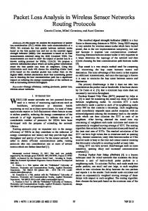
2.1 Examples Single-hop packet combining. In a standard ARQ system, the receiver immediately discards a packet received with errors. Hybrid ARQ (HARQ) schemes improve upon ARQ by buffering a corrupt packet at the receiver whilst awaiting retransmission, and combining multiple corrupt copies to do error recovery. The idea of HARQ originated in the work of Sindhu [20], who first considered the idea of merging two non-coded packets to correct errors. Rather than retransmit the original packet as is, the sender may retransmit the parity bits produced by applying an encoding operation to the original packet. This allows the packet combining decoder to recover from more errors than if the same bits had been transmitted twice. The idea of using plain and parity packets, which we employ in this paper, has been studied in various forms using increasingly complex codes [14] [7]. The contribution of this work is to generalize the ideas of hybrid ARQ to multi-hop primitives and apply them in a practical setting. Multi-hop packet combining. When a packet traverses a multi-hop route, HARQ may happen on a hop-by-hop basis anywhere along the path. But beyond this, packet combining also enables a novel form of multi-point interaction that occurs whenever an upstream node beyond next hop overhears a corrupt packet. This corrupt packet is buffered and used for error correction when the next hop forwards the packet. By exploiting this multi-point interaction in addition to single-hop combining, the effect of packet combining on a route is greater than the sum of packet combining on constituent hops. The top row of Fig. 1 depicts a three-hop route with a sender A, relays B and C, and destination D. In Fig. 1(b), the sender transmits a packet to B, who receives it without error. Though the link from A to C is too lossy to be used by the protocol, it still delivers a large number of corrupt packets, and C receives a corrupt copy of this packet. In Fig. 1(c), node B forwards the packet, which is received with errors at C. Since C now has two corrupt copies of the packet (one sent by A, one by B) it can combine them and (with some probability) recover the original packet. Finally C forwards the packet which arrives with errors at D, who now has three

corrupt copies and recovers the packet by combining them. Note that C may occasionally overhear A’s packet without errors. The use of an opportunistic routing protocol that can exploit such packets (e.g., [2]) is orthogonal to packet combining, and both may be used in complement. We should emphasize that no network layer state need be exposed to the packet combining layer; this layer simply accepts corrupt packets blindly and attempts to combine them, without using topological information from the network layer. Broadcast Packet Combining. We now turn to the network broadcast primitive, where one node seeks to disseminate a packet to all others. We consider a simple flooding protocol that forwards each flooded packet once (with duplicate detection by a sequence number or random identifier). Other, more efficient approaches to broadcasting are possible [13] [8]. We note that packet combining can enhance other broadcasting protocols in a manner similar to flooding, and study flooding because it is a simple mechanism found in many applications (such as Surge, tinyDB [15], or directed diffusion [10]). Fig. 1(e) shows a 5-node topology. In Fig. 1(f), node A originates a flood packet that is received without errors by B, and with some errors by C and D. B now transmits the packet (Fig. 1(g) ); it is received with errors by nodes E and D. Node D now has two error copies of the same packet, from which the packet combiner decodes the original packet. Finally in Fig. 1(h), node D transmits the packet. Node C receives the packet without errors, and can therefore discard the corrupt packet held in its buffer. Node E however receives a corrupt packet, and combines the two previous corrupt copies to correct the errors. Unlike multi-hop routing, flooding never uses link-layer retransmissions, and therefore cannot benefit from the singlehop interaction of HARQ. However packet combining can take advantage of a larger number of bad packets in flooding than routing, since a bad packet received at any node may be exploited (Table 1).

2.2 Comparison with FEC An alternative solution to packet combining would be to use standard FEC techniques. It is therefore natural to ask: Why not use FEC instead of packet combining? The answer is two-fold. The first part concerns link variability. For any link with known and stationary error characteristics (biterror rate, burstiness), one can design a channel code which optimally matches those characteristics. However, as soon as the link deviates from the characteristics the code was designed for, then performance drops sharply: if the link is more error-prone than expected the code cannot recover the errors, and if it is better than expected, transmitting parity bits becomes redundant overhead. In particular, appending any error-correcting bits to a packet which arrives without errors is highly wasteful. Sensor network measurement studies [25] [5] have shown that link variability is high both in time and across space, in particular for those very links which are error-prone and most require FEC. Therefore, it is difficult to design an efficient static FEC system for the wide range of channel conditions seen in a sensor network. Adaptive FEC can provide a solution to time-varying channel conditions, but requires frequent, costly channel measurements to obtain a timely and accurate estimate of the channel biterror rate. These measurements are especially costly when the traffic rate is low and the channel potentially changes between every packet transmission. In comparison, packet

combining provides a simple form of adaptive channel coding that requires no explicit channel measurements: if the channel is good, the initial transmission is received correctly with no redundant error correction bits having been transmitted. If the channel is poor, then the retransmission needs only to contain additional error-correction bits to “elevate” the two combined packets at the receiver to a lower-rate code, with which more errors can be corrected. The second part of the answer is that packet combining naturally transposes to multi-hop scenarios, whereas FEC is inherently geared toward point-to-point links. In the case of multi-hop routing, FEC can improve the performance of each individual links, but can not take advantage of overheard corrupt packets at downstream nodes. In contrast, packet combining can do both. In the case of broadcasting, a node receiving multiple corrupt copies from different nodes can not combine them with standard FEC.

3.

CHANNEL MEASUREMENTS

Before designing any error correction system, it is necessary to know the error characteristics of the channel being addressed. In the case of packet combining, we are interested in the following two aspects: • Error characteristics: What bit error rates do we see in corrupt packets? How bursty are error patterns? We will see that error characteristics are such that a simple channel code can already correct a large number of error patterns. • Sources of packet loss: What portion of packet loss is due to packets that are received corrupt and discarded by the link layer, and what portion is due to missed packets, i.e., those packets that were not received at all? This breakdown is critical: if loss is primarily attributable to missed packets, then an errorcorrection scheme will see too few corrupt packets to be effective. These measurements motivated the design of a new error-tolerant preamble detection scheme (ETPD) that we present in the final part of this section. We consider an asynchronous, random-access channel. A known preamble pattern, serving to achieve receiver synchronization, precedes each transmitted packet. A node in receive mode continuously draws in bits from the radio until the previously received bits exactly match the preamble sequence; once a preamble has been detected the full packet is drawn in. If a preamble is received with any bit errors, then entire packet is missed1 . The notations are as follows: • pd is the probability of error-free packet delivery. • pc is the probability of corrupt packet delivery (packet received with one or more bit errors). • pm = 1 − pd − pc is the probability of missed packet (packet not received at all, because the preamble was mis-detected). We therefore have pm + pd + pc = 1, and the overall packet loss probability is pc + pm . • Rcm = pc /pm is the ratio of corrupt to missed packets. Packet combining will work better with high values of Rcm ; the ideal case is when pm is close to 0. • Lpre , L, and Ltot = Lpre +L are respectively the preamble length, packet length (including headers and payload), and total transmission length, in bits. 1 This mechanism is used in 802.11 and 802.15.4 as well as non-standard radios like the CC1000.

A

C

B

D

A

C

B

a)

D

A

B

C

C

A

D

a)

E

: good link

b) : intermediate link

B

C

A

C

A

D

B

D

B

B

c)

E

d)

E

: poor link

D

C

d)

D

B

A

c)

b)

A

D

C

: error−free packet

E

: packet with errors

Figure 1: Packet combining in multi-hop primitives. Top: multi-hop routing. Bottom: network broadcasting.

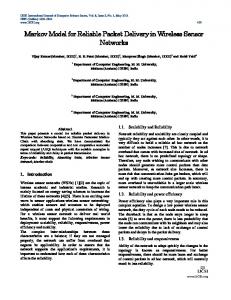
3.1 Bit-level Error Measurements We now examine the error characteristics of our channel, starting with the number of bit error rates observed in corrupt packets. Figure 2(a) shows the distribution of BER over all corrupt packets. Most corrupt packets have few bit errors: the proportion of corrupt packets with a bit error rate below 0.05 is 85% both for short and long packets. The proportion of packets with a bit error rate greater than 0.1 is 6% for short packets and 10% for long packets. With two or more corrupt copies of a packet, we effectively have an encoding that is half-rate or lower. Bit error rates of 0.05 are within corrective reach of half-rate codes [14]. This indicates that many corrupt packets should be recoverable through packet combining. But bit error rate alone does not completely characterize the error process; in particular burstiness is an important factor to guide the choice of errorcorrection mechanism. Assume for example the use of a code

P(ei+k | ei)

0.1 0.08 0.06 0.04 0.02 0 1

5

10

15

20

25

30

35

40

45

50

40

45

50

40

45

50

Indoor (Packets with BER < 0.05) P(ei+k | ei)

We used two testbeds: a 39-node indoor testbed with nodes attached to the ceilings across several offices on one floor of UCLA’s Boelter Hall and a 10-node outdoor testbed installed in a UCLA courtyard. Each node is a Crossbow Mica2dot, which has an Atmel ATmega128L microcontroller with 4KB of RAM, 128KB of Flash, and a CC1000 radio [6]. The radio operates in the 433Mhz band, uses narrowband 2-FSK modulation, and runs at a bit rate of 19.2Kbps (bits are Manchester encoded, resulting in a 38.4kbps symbol rate). In our experiments each node was in turn the sender; other nodes listened and logged received packets via a wired backchannel. We ran experiments varying two parameters: transmission power (-15dBm and -5dBm) and packet length (16 and 128-byte payloads, with a 5 byte header and a 2 byte trailer), giving us a total of four configurations and 150,000 packets transmitted. Error characteristics are very different on a congested network, where a large number of errors are due to interference bursts from concurrent transmissions, and on a network with low channel occupancy. Our aim is to improve performance of low-power, low-rate applications, and we consequently made measurements on a “silent” network with no concurrent background traffic. Note that in the presence of external RF sources (other wireless devices, electronics), burst interferences are still possible even in a silent network.

Outdoor (Packets with BER < 0.05)

0.1 0.08 0.06 0.04 0.02 0 1

5

10

15

20

25

30

35

Indoor (Packets with BER > 0.05) P(ei+k | ei)

ˆ cm ) denotes the estimated value • pˆd (resp. pˆc , pˆm , and R of pd (resp. pc , pm and Rcm ) made on the empirical data for a given link.

1 0.8 0.6 0.4 0.2 0 1

5

10

15

20

25 30 Lag k (bits)

35

Figure 3: Empirical bit-error probability conditional on an error having occurred k bits earlier. Horizontal lines show the average bit-error rate for each data set. Top and center: packets with BER < 0.05. Bottom: packets with BER > 0.05. which can correct 1 error in every 8-bit codeword, and a BER well below 1/8. If errors are uniformly distributed, then most codewords will have 0 or 1 errors and will be recovered. For the same BER, but with bursty errors, the probability of a packet containing a uncorrectable codeword with more than one error is increased. Figure 3 shows the empirical bit-error probability conditional on an error having occurred K bits earlier. Horizontal lines show the average bit-error rate for each data set, or equivalently, the auto-conditional error probability of an i.i.d. error process with same BER. These plots suggest that one can coarsely classify corrupt packets into two categories: packets with a low bit-error rate and low error burstiness, and packets with higher error rates and a bursty error process. Since the former category represents nearly 90% of all corrupt packets, (see Fig. 2(a)) and since the latter has higher error rates which are harder to correct with low computational complexity, we design Section 4 an errorcorrection coding which is designed to correct the low BER majority of packets, but not the highly bursty ones.

Empirical CDF of Rcm

Empirical CDF of Rcm with error-tolerant preamble detection 1

0.9

0.9

0.9

0.8

0.8

0.7

0.7

0.8 0.7 0.6 0.5

0.2

0.6 0.5 0.4 0.3

0.4 0.3

P(Rcm < x)

1

P(Rcm < x)

P(BER < x | BER > 0)

Empirical CDF of bit error rates 1

0.05 0.1 0.15 0.2 0.25 0.3 0.35 0.4 0.45 0.5 BER

0.5 0.4 0.3

16 byte payload (all links) 128 byte payload (all links) 16 byte payload (weak links only) 128 byte payload (weak links only)

0.2 Outdoor Indoor

0.6

0.1 0 1

5

10 x

15

Ne = 0 Ne = 1 Ne = 2 Ne = 3

0.2 0.1 20

0 0.01

0.1

1

10

100

1000

x

ˆ cm , the ratio of a) Empirical CDF of bit error rates. b) Empirical CDF of R Most corrupt packets have few bit errors. corrupt to missed packets.

ˆ cm with c) Empirical CDF of R error-tolerant preamble detection.

Figure 2: Bit error rate and preamble detection measurements. The top and center plots are computed over the subset of packets with BER < 0.05. Of these two plots, the outdoor is least bursty: the presence of an error at bit i slightly increases the probability of errors in the following two bits, but after that the error probability is the same as for an i.i.d. process. The indoor trace is slightly more bursty, with the probability of an error immediately following a previous one at approximately 0.09. This difference between indoor and outdoor burstiness, may be due to interfering RF sources which are more likely to be found inside a building than outside. The bottom plot is computed over the much smaller subset of packets with BER > 0.05. Here, the picture changes sharply: the error process is much more bursty, over a range of at least 50 bits. For these packets, the short code discussed above would not suffice, since the probability of at least one codeword in the packet having multiple errors is high. While we have chosen, due to complexity constraints, to “ignore” the class of packets with highly bursty errors, we note that two simple techniques are possible two improve error correction with bursty errors. The first is interleaving. The second is to use codes with block lengths larger than the burst lengths. Unfortunately, it is not feasible to implement either technique in software with simple microcontrollers. For increased burst-tolerance and robustness, both interleaving and longer-block decoding are possible in a hardware implementation.

3.2 Sources of Packet Loss and ETPD We now turn to the breakdown of packet loss between corrupt and missed packets. Fig. 2(b) shows the empirical ˆ cm , the observed ratio of corrupt to missed packets, CDF of R ˆ cm is lower for for short and long packets. We observe that R short packets than for long packets. For example no links ˆ cm > 5 with short packets, whereas with long packets have R ˆ cm > 5. This observation can be over 40% of our links have R explained by noting that pm is independent of packet length (because preamble length is constant), whereas pc increases with packet length, since for a given BER, the probability that at least one bit in the packet is corrupt increases with the number of bits. From this observation, we expect packet combining to give more gains with long than short packets. ˆ cm over weak links, which Fig. 2(b) further distinguishes R ˆ cm is lower when conwe defined as those with pˆd < 0.4. R sidering only the weak links. Yet, links with a low delivery rate are those where packet combining is most needed, and if packet combining sees too few corrupt packets its utility

will be limited. Since a receiver misses a packet whenever its preamble is received with errors, these measurements motivated the design of ETPD, to increase Rcm by allowing the reception of a packet in the presence of preamble bit errors. Our initial implementation of ETPD accepted preambles p with up to Nmax = 4 bit errors (out of 4 preamble bytes). p We set this initial value for Nmax because packets with more preamble errors are likely to have too high a bit error rate to be corrected with a half-rate code, and furthermore allowing a greater number of errors would increase the probability of false positives. We added the additional constraint that no single byte could have more than 1 bit errors, to further reduce the probability of false positives and allow for more efficient software implementation. We ran experiments identical to those of Section 3.1, except that the received preamble was also dumped out along with each packet. We then classified received packets according to the number Ne of preamble bit errors. Figure ˆ cm with and without 2(c) compares the empirical CDF of R ETPD for 1 ≤ Nep ≤ 4. The data for all CDFs originate from the same packet traces: by examining the received preambles, we can see which packets would be received with a given preamble error-tolerance. ETPD allows a significant ˆ cm : we go from having R ˆ cm > 10 for only 20% increase in R of links without ETPD, to 60-70% with ETPD (depending on the setting of Nep ). ˆ cm does not demonstrate alone The observed increase in R that ETPD is worthwhile. Under the assumption that the channel does not vary dramatically over the duration of a packet, we expect that packets with error(s) in the preamble will have a higher bit-error rate than those without. If those packets have a sharply increased BER, then receiving them may be pointless. We therefore classified corrupt packets by the number of preamble errors each one had, and computed in Table 2 the observed bit-error rate for each set of corrupt packets. This table shows that the packet BER increases with the preamble BER, in line with the intuition that BER does not vary widely over the duration of a packet. Our final ETPD implementation can be configured for p maximum allowed preamble errors Nmax between 0 and 3. p We set Nmax = 2 for all further experiments reported in this paper, since with higher error tolerance, the marginal increase in packet yield is small (Fig. 2(c)), and the additional packets have a very high bit error rate (Table 2). A final aspect to consider with ETPD concerns the increased probability of false positive preamble detections. When placed in receive mode, a radio transceiver continu-

Nep 0 1 2 3

Preamble BER Nep /Lpre 0 0.031 0.063 0.094

Packet BER (L = 16) 0.029 0.052 0.073 0.095

(L = 128) 0.032 0.084 0.128 0.165

Table 2: Observed bit-error rate as a function of number of preamble bit errors Nep , for two different payload lengths L. ously reads and demodulates bits from the RF front-end. If no transmission is ongoing, this effectively amounts to reading random bytes. By increasing the preamble detection’s error-tolerance, we increase the probability of having a sequence of random bytes that is falsely detected as a preamble. We must therefore take into account the probability of spurious packet receptions due to false positive preamble detections. The probability of a spurious reception P (Nep ), when tolerating exactly Nep errors in the preamble can be simply computed by counting the number of possible 32 bit sequences with Nep errors, and no more than 1 error per Pi=N p ` p ´ p byte: P (Nep ) = 2−32 i=0 e N4e 8Ne . For our chosen setp ting Nmax = 2, this evaluates to a probability on the order of 10−7 , meaning that the number of spurious packet receptions occurring in practice is negligible.

4.

DECODING AND MERGING

Section 2 showed how a node may come to receive corrupt packets in various settings. We now describe the packet combining algorithms used on the receive path and the corresponding packet encoding functions on the transmit path.

4.1 Linear Block Codes The class of error-correcting codes is vast. We focus in this work on linear block codes, which can be implemented efficiently in software using table-based methods (unlike, for example, convolutional codes). A (n, k) linear block code is defined by its generator matrix G, of size k x n. The encoder multiplies each input block with the matrix G, transforming k input bits into a codeword of length n. The decoder, given a received codeword of n bits, finds the closest codeword (in the set generated by G) and returns the information bits corresponding to that codeword. If the number of bit errors is higher than the half-distance between two codewords, then the decoder returns the wrong information bits (that can then be detected with high probability by an outer CRC checksum). If two closest codewords are at equal distance to the received word, the decoder cannot infer which was the transmitted codeword, and declares a failure. For a general overview of decoding algorithms, we refer to [14]. Within the class of linear block codes, we further restrict our attention to invertible and systematic linear block codes. A block code is systematic if the first k bits of a codeword are the same as the input message bits, in other words the generator matrix of a systematic code is of the form G = [I|P ] where I is the k × k identity matrix and P is a k × (n− k) matrix called the parity matrix. A block code is invertible if n = 2k and the matrix P is invertible. Note that an invertible code is half-rate since n = 2k. Given this matrix P , and an input word m (of length k bits), the encoder outputs the 2k-bit codeword Gm = [I|P ]m = [m|P m]. This codeword is the concatenation of the unmodified input m,

1

2

3

1

2

3

... ...

n

Corrupt plain packet

n

Corrupt parity packet

Plain and parity blocks are interleaved and passed to the decoder. ... 1

1

2

1

2

2

3

3

3

...

n

n

n

Figure 4: Packet Decoding: Recovering the original packet from two corrupt packets, when one is plain and the other is parity. which we call the plain bits, and P m, which we call the parity bits. Note that since P is invertible, there is a oneto-one mapping from P m back to m, and therefore one can recover the plain bits from the parity bits of a codeword and vice-versa.

4.2 Packet Encoding and Decoding In a standard block-coded FEC system, the encoder transmits the plain and parity bits of a codeword together. This comes at the expense of increasing the number of transmitted bits by a factor of two, in the case of a half-rate code. As discussed in Section 2.2, imposing this overhead on every packet transmissions is prohibitive, given that many packets are received without errors and do not need parity bits. The key intuition allowing to use a code without transmitting redundant overhead is to observe that we can simply send some “plain” packets which are not encoded, and some “parity” transmissions containing only the parity part of each codeword. Specifically, consider an input packet m = m1 m2 . . . ml , where each block mi is of length k bits. The encoder outputs either m unmodified (a plain packet), or the packet m∗ = P m1 P m2 . . . P ml (a parity packet). How the encoder chooses between outputting a plain or a parity packet is discussed in Section 4.4. The motivation for using a systematic, invertible code is now apparent: 1) If a parity packet m∗ is received without errors, the original m is obtained simply by multiplying the packet by P −1 : P −1 m∗ = P −1 P m1 P −1 P m2 . . . P −1 P ml = m1 m2 . . . ml = m. Note that since a parity packet has the same length as the corresponding plain packet, the system does not transmit any redundant overhead on good links, whether it transmits a plain or a parity packet. 2) Two corrupt copies of a packet (one plain and one parity) can be jointly decoded by taking k bits at a time from each packet, and decoding the concatenated word. This operation is illustrated in Fig. 4. Our implementation uses the Hamming (7, 4) code, extended to (8, 4) with an additional error-detecting bit. The (7, 4) code can correct up to one error per 7-bit block; the extended (8, 4) code allows in addition to detect (but not correct) any 2 bit error per 8-bit block. The primary motivation for using the extended code was to have byte-aligned blocks, given that unaligned operations are inefficient to implement in software. The additional error detection capability of the extended code allows the decoding operation to ’abort’ as soon as it encounters an uncorrectable error, in which case wasted CPU cycles are saved.

0 00 0 0 0 00 0 0 0 0

000 0 0 0 01 10 0 0

Transmitted data packet

Two received corrupt packets

000 1 0 0 01 10 0 0 000 0 0 0 00 10 0 0

000 1 0 0 00 10 0 0 000 0 0 0 0 1 00 0 0

000 1 0 0 00 00 0 0

000 1 0 0 01 00 0 0 000 0 0 0 00 00 0 0

Set of candidate packets considered by packet merging

Figure 5: Packet Merging: Recovering the original packet from two corrupt packets of same type. Our choice of a short code was dictated by the practical constraints on decoding overhead: the most efficient software implementation is based on table-lookups, and table size is exponential in block length. With more processing power, syndrome decoding would alleviate these memory requirements. Beyond this constraint, any other systematic and invertible block code can be used with minimal modifications. For example a longer Hamming code, an extended Golay code (with block length 24), or a Reed-Solomon code all have more error-correcting power than the Hamming (8, 4) we used.

4.3 Packet Merging The preceding section showed how two corrupt packets of different types (one plain, one parity) are jointly decoded. What if the receiver has two corrupt packets of same type? We call the corresponding operation packet merging. Given that it essentially corresponds to decoding a repetition code, it is not surprising that merging can correct fewer errors than decoding. Let m1 and m2 be corrupt copies of an original packet m; ie m1 = m + e1 and m2 = m + e2 , where e1 6= 0, e2 6= 0, and additional is modulo 2. Note that m1 + m2 = e1 + e2 . Therefore by XORing m1 and m2 , the receiver obtains a merged error mask with a 1 in all bits that are errors in either m1 or m2 . Note that the merged error mask does not show an error bit that occurred in identical positions in both packets. We call such an error a hidden error. Assume that the merged error mask contains ne non-zero bits. There are then 2ne − 2 candidate error patterns that may have occurred. The packet merging procedure corrects each candidate error pattern on one of the corrupt packets, and recomputes the checksum to verify if it matches the transmitted CRC checksum in the packet trailer2 . Figure 5 illustrates a case with ne = 3 and shows all 23 − 2 candidate corrected packets. We distinguish three cases, based on the number k of error patterns for which the checksum is valid: k = 0. None of the candidate error patterns, corrected on the corrupt packet, yield a valid checksum. Packet merging cannot recover the original packet. This case can only happen if there are hidden errors, since otherwise of the candidate error patterns corresponds to the effective error pattern. k = 1. A unique error pattern yields a valid checksum. The resulting packet is passed up the stack. k > 1. Multiple error patterns can recover a packet with a valid checksum. Which (if any) corrected packet is the original packet is undecidable; a failure is declared. Since the number of candidate error patterns increases exponentially with ne , the computational overhead becomes 2

Merging is not attempted if the two received packets have differing checksums, since this means that either both packets are different (in which case combining is pointless), or that one of the checksums has errors, and we cannot know which (if any) is correct.

prohibitive if we attempt to merge two packets that differ in a large number of bits. The probability of hidden errors increases with ne , and furthermore, so does the probability of the case k > 1 occurring. We can see this intuitively by considering the extreme case where both packets differ in all bits, in which case we would iterate through all 2L possible packets. For these reasons, we introduce an algorithm parameter nmax that upper-bounds the largest value of ne for which packet merging is attempted. If the merged error mask contains more than nmax errors, merging is not attempted and a failure is declared. Besides bounding the number of candidate packets searched, this parameter also controls the two key performance metrics that are probability of merging success, and probability of false positives. We shall see in Section 5 that the effective choice in our implementation is dictated by the computational constraints of merging more than the probability of false positives. For a given set of parameters (bit error rate, packet length), the error correction performance of this merging algorithm is characterized by two measures. The first is the probability of success (the original packet is correctly recovered from two corrupt copies), and second the probability of false positives (the algorithm produces a ’repaired’ packet that is different than the original packet, but for which the checksum is correct). Clearly we wish to maximize probability of success whilst minimizing probability of false positives. Note that even without packet merging, the probability of false positives is never zero, because a CRC checksum cannot detect every possible error pattern. The key is then to ensure that merging does not significantly increase the probability of false positives with respect to a standard receiver. Merging increases the probability of false positives by at most a factor of 2nmax . Note that in the absence of hidden errors, the error pattern that effectively occurred is present in the set of candidates. Therefore a false positive can only occur in the presence of hidden errors: if there are no hidden errors, and if there is an additional ’false positive’ error pattern giving the correct checksum is correct, then the algorithm finds more than one candidate repaired packet and declares a failure (case k > 1). This further reduces the probability by a factor of at least nmax /L.

4.3.1 Decoding and merging failure probability We consider i.i.d. bit errors with bit error probability pe . With the (8, 4) Hamming code which can correct up to one error per codeword, jointly decoding two packets fails if any codeword has more than one error. The decoding failure probability ρ is thus: ρ = 1 − ((1 − pe )8 + 8pe (1 − pe )7 )L/4 .

(1)

where the the exponent is L/4 because the decoder operates over two packets of length L bits, or equivalently L/4 codewords of 8 bits each. Merging fails in the presence of hidden errors or when both corrupt copies contain together more than nmax errors. For simplicity, we approximate the probability ρ˜ of this event by the probability that two corrupt packets contain less than nmax errors, noting that the probability of hidden errors approaches 0 for small values of nmax . ! nX max 2L ρ˜ = 1 − pe i (1 − pe )2Lpkt−n (2) i i=0

4.3.2 Efficient CRC computation The overhead of the CRC computation is critical, because for each candidate error pattern, packet merging must recompute the CRC on the packet corrected with the error pattern. For example, in MRD [16] the CRC is computed in a non-incremental fashion, and was found to be the bottleneck for the entire combining process. Since the set of bits that change between each candidate packet is small (at most nmax ), recomputing the CRC over the entire packet is redundant. However, existing incremental CRC algorithms (such as those for ATM/IP networks [3]) do not apply here because they assume that only bits at fixed positions (in packet headers) can change at each hop. In our case, the candidate errors can be anywhere in the packet. We now describe an incremental algorithm that recomputes the CRC on a packet with one operation per changed bit. It can be seen as a extension of [3] which removes any constraints on the changed bit’s location in the packet. We denote, as polynomials over GF(2), the packet M (x), and E(x) the candidate errors bits (for which we wish to recompute the CRC), we would like to compute the CRC over the message M c (x) = M (x) + E(x): xr (M (x) + E(x)) mod G(x) = x M (x) mod G(x) + xr E(x) mod G(x), | {z } | {z } r

f ixed

(3)

variable

where G(x) is the CRC generator. The separation of (3) into a sum is possible because the CRC is linear. Defining Ek (x) as the vector containing a single 1 at position k and zeros elsewhere, we can further decompose the variable part of (3) as xr E(x)

mod G(x) =

L X

1i (xr Ei (x)

mod G(x)),

(4)

i=0

where the indicator variable 1i is equal to 1 iff E(x) contains a 1 at bit i. So with a pre-computed lookup table T with entries defined as T [i] = xr Ei (x) mod G(x), we can recompute the CRC in one operation per changed bit. The table T has length L and can be stored in ROM; in exchange we make a linear gain of L/ne in computational overhead. As the profiling results of Section 5.1 will show, packet merging would be computationally infeasible (in software) without this reduction.

4.4 When to send a plain or parity packet Decoding can correct more errors than merging, and uses fewer CPU cycles (as we shall see in Section 5.1). We therefore wish to maximize the probability that two corrupt packets received successively at a node are of different types (plain and parity), so that they can be decoded. In the case of retransmissions, this is straightforward: the sender alternates between parity and plain. For multi-hop and flooding however, there are multiple potential receivers, and the sender cannot know the type of any corrupt packets already buffered at a neighbor. For a node relaying a multi-hop packet, the initial transmission is of opposite type to the last received packet. For a flooded packet, the sender randomly chooses between plain or parity. Receiver processing depends on the type of packet received. A valid plain packet is passed directly up the stack; a valid parity packet must first be inverted. Two corrupt packets of same type are merged, and then inverted if they

m Plain Parity

Action None Invert

m Plain Plain Parity Parity

a)

n Plain Parity Plain Parity b)

Action Merge Decode Decode Merge, invert

Table 3: Receiver processing actions: a) for a valid packet m, b) for two corrupt packets m and n. are parity; two corrupt packets of different type are decoded. These actions are summarized in Table 3.

4.5 Extensions Two simple improvements can be made to the current design. We outline them for completeness and note that they can be implemented as extensions to SPaC. The first is to allow the receiver to buffer more than two corrupt packets. With multiple corrupt copies, the receiver has more candidate pairs to combine.` The ´ probability of successful combining thus increases as n2 , where n is the number of packets at hand. Note however that this also implies an increase in the worst-case computational cost. The second improvement is to use a higher order (mn, n) code with a generator matrix of form G = [G1 |G2 | . . . |Gm ], where each Gi is an invertible matrix of dimension n × n. This generalizes the notion of plain and parity packets to m distinct packet types, each being invertible in the absence of errors. A further desirable property is that any two submatrices taken together form a half-rate invertible code such as the ones considered previously in this section, so that the combiner can jointly decode any two packets of different types. With all m packets of distinct types, the encoding rate 1/m allows to correct yet more errors. The general form of such codes is not known, but some specific examples exist such as the work of Alfaro and Meo [7], who propose a third-order (24, 8) code. Though the 24-bit block length means that decoding three packets jointly would be hard in software on sensor nodes, such a code is advantageous even if we only decode two packets at a time (giving a (16, 8) code), because it decreases likelihood that any two corrupt packets are of same type. With such a code, merging operations are attempted less frequently and the combining success rate is increased.

5.

IMPLEMENTATION

We implemented ETPD and SPaC in TinyOS. The SPaC component currently works over B-MAC; it uses simple packet interfaces, and can be integrated with other link layers such as S-MAC [23] or T-MAC [22] with minimal modifications. The ETPD implementation is part of the lowest part of the MAC and is not cleanly portable. We embed the type of each packet (parity or plain) in the preamble so that it does not require additional bits. Fig. 6 shows a high-level block diagram of the necessary functions. Link-layer acknowledgement and retransmission functions are shown for completeness. Shaded components are those required to support SPaC; white components are also present in a non-packet combining system. On the send path, the inner encoder block implements the plain/parity decision of section 4.4. On the receive path, the combiner block performs decoding or merging depending on the types of the input packets. The receive path decision sequence is represented in Fig. 7.

Upper layers Inner Encoder

Outer Encoder (CRC)

Retransmission Buffer

Component ETPD Pkt Combining

Data packets

Feedback (ACKs)

RAM 8 2L + 78

ROM (code) 450 3674

ROM (tables) 256 16L + 512

Table 4: Memory footprint in bytes, as a function of maximum packet size L.

Transmitter

Data packets

Feedback (ACKs)

Outer Decoder (CRC) Corrupt Pkt Buffer

Upper layers

Function Encode/Invert Decode Diff Merge (ne = 2) Merge (ne = 4) Merge (ne = 6)

Inverter

Combiner

Receiver

Figure 6: Block diagram of packet combining functions on transmit/receive paths.

Figure 7: Receiver Flowchart. Buffer management. Given two received corrupt packets, a node does not know if they correspond to the same original packet, or two different packets. A buffer management strategy is therefore important to reduce the number of attempts to combine two different packets. The current implementation records a timestamp with each received corrupt packet, and discards a corrupt packet after a given timeout, which is determined based on the traffic load and statically configured into the application. Note also that combining is not attempted for packets with differing CRCs (except for multi-hop packets). There are no explicit mechanisms to detect if two corrupt packets come from different originals – whenever the receiver has two corrupt packets, combining is attempted. This means that combining two different packets, which will fail and is a waste of CPU cycles, can sometimes happen. Our assumption of a low-rate application is key to this design choice: with a short enough timeout, cache pollution and cross-traffic (where two different corrupt packets arrive in a smaller interval than the timeout value) are infrequent.

CPU Cycles L=29 bytes 128 436 1673 2155 9234 1228 4396 172 172 1563 1563 9305 9305

Equivalent transmitted bits 29 128 1.1 4.3 5.6 24.1 3.2 11.4 0.5 0.5 4.1 4.1 24.2 24.2

Table 5: Worst-case CPU overhead of SPaC functions. The CPU energy used for each function is compared with the number of bits that the radio would transmit to use equivalent energy. More sophisticated buffer management strategies are possible. For example, determining the timeout adaptively, or not buffering a corrupt packet that can only be sent once (such as local broadcast packets sent by a routing protocol). Another option would be to add a randomly chosen identifier (with error protection) to each packet, but the overhead of adding a fixed field to each packet would outweigh the gain from making a few less unnecessary combining attempts. Multi-hop packets. Routing headers on multi-hop packets usually contain fields that change at each hop, such as nexthop address or distance to destination. Combining packets with differing contents would fail, and so it is necessary to take into account the header fields which may change at each hop. Our current implementation treats multi-hop packets differently from single-hop and broadcast packets, and ignores these fields from the CRC and combining operations. A future improvement will consist of applying the incremental CRC to the modified fields rather than ignoring them. Memory Footprint. Wherever possible, we used precomputed table lookups for encoding, decoding and merging. The memory overhead depends on the maximum packet length defined for the application. With the default value of 29 bytes, the ROM footprint of our implementation is 5580 bytes, including code and lookup tables. The RAM footprint includes two packet buffers and totals 158 bytes. A detailed breakdown is given in Table 4.

5.1 CPU Overhead We evaluated the CPU overhead of all packet combining functions using a combination of manual inspection and scripts that we derived from the PowerTossim [19] distribution. We also converted the computation cost of each function into equivalent communication cost3 to allow easy comparison between CPU and radio energy costs. The scripts disassembled the binary image (compiled at -O3 gcc optimization level) and annotated each line in the c sources with the number of corresponding CPU cycles. When a line or function was inlined at different places in the 3

This translation was computed for the case where the radio sends at 0 dBm, using the constants measured in [19]; converting to other transmit powers is simply a matter of multiplying the cycle count by a different constant.

6.

EVALUATION

In this section we present performance results for the three networking primitives of Section 2 (single-hop with retransmissions, multi-hop routing, and flooding), as well as endto-end results on a live network. The results in this Section cover the two testbeds of Section 3, as well as a 5-node testbed and a semi-permanent deployment, both at EPFL’s BC building. Three very different physical environments have therefore been considered; while they cover a substantial ground they are by no means exhaustive.

6.1 Single-hop with Retransmissions We used B-MAC’s acknowledgement mechanism with sender-side ACK timeouts increased by 2 radio byte transmission periods to account for the increased receiver processing time (this results in a maximum throughput reduction of less than 4%, in the worst-case where the receiver must merge every two packets with ne = 6). We built a simple retransmission scheme based on the acknowledgement mechanism that is implemented in B-MAC. When acknowledgements are enabled, a node acknowledges reception of a valid unicast packet addressed to it by transmitting a short (4 byte) “ack” code. The sender waits a short period for

Throughput efficiency versus underlying link PDR 1

16-byte payloads Theoretical 128-byte payloads Theoretical

0.9 0.8 0.7 0.6 η

assembly code, with different cycle counts, the script computed the average of the different counts. We then manually summed the total cycles for each function, being careful to account properly for loops (counting the initialization assembly once, and the loop test as many times as the loop is executed). For most functions, the cycle count depends on the input packets and error patterns. For example, in the case of a packet merging, the procedure exits early if it encounters two candidate error patterns resulting in the same CRC (case k > 1, Section 4.3), or yet earlier if the merged error mask has more than nmax errors. In the case of a packet decoding, the decoding loop exits early if the (8, 4) Hamming code detects an uncorrectable error. We present here the worst-case cycle counts for all functions with input-dependent behavior. Table 5 shows worst-case cycles and energy-equivalent radio transmitted bits for each function. Encoding, inverting, and decoding are linear in packet size. Encoding and inverting use negligible CPU energy in comparison to transmission, representing less than 0.5% of the energy to transmit the packet. Decoding is barely more costly in CPU energy, requiring less than 2.5% of a packet transmission cost. Merging two packets requires first a “diff” operation to compute the merged error mask (Section 4.3) by XORing two packets. It is then followed by a search through all candidate error patterns and has cost exponential in ne . The overhead of merging is sharply higher than that of other functions. We set nmax = 6 in our experiments, as the worst-case overhead for ne > 6 becomes non-negligible in comparison with a packet transmission cost. For ne = 6, merging is comparable to 7% of the transmission cost for a packet with 29 byte payload, or 2% with a 128 byte payload. In summary, the energy overhead of SPaC shown by these measurements is far lower than the energy cost of sending a packet, even with the worst-case numbers given in this section. It is nonetheless not negligible, in particular when considering the simplicity of the codes used and the tabledriven implementation; computation must therefore be carefully considered in the design of more future, more complex schemes.

0.5 0.4 0.3 0.2 0.1 0 0

0.1

0.2

0.3

0.4

0.5 pd

0.6

0.7

0.8

0.9

1

Figure 8: Single-hop throughput efficiency η as a function of raw throughput efficiency pd . the acknowledgement, and sets the packet ack field appropriately before signalling the sendDone() event, allowing the upper layer to take some action (e.g., retransmit the packet) if the packet is unacknowledged. We define the single-hop throughput efficiency η (or simply throughput) as 1/Nt , where Nt is the average number of packets transmitted until the packet is successfully accepted at the receiver. The throughput without combining is therefore pd . The retransmission mechanism retransmits a packet up to a maximum number of attempts Tmax , until a transmission is positively received. We set Tmax = 5 for the experiments of this section. We ran these experiments over 20 pairwise links (using a 5-node subset of the testbed), with varying transmission power and packet lengths. Nodes dumped all sent and received packets via the serial backchannel, as for our bit-level measurements. When a node successfully combined two corrupt packets into a valid one, this packet was also logged, allowing us to distinguish in the logs which valid packets were the result of a combining operation. In addition, the sender logs showed how many retransmissions were needed for each sent packet. Fig. 8 shows the observed throughput efficiency η as a function of underlying link delivery pd , as well as the theoretical curve from Appendix A. The theoretical curve qualitatively matches the empirical data, and is a good approximation for pd > 0.6. For lower values of pd , the theoretical curve has an upward bias. This is due, at least in part, to the finite number of retransmissions Tmax used in the experiments. The empirical results show that many links with a raw PDR of 5-20% see a throughput increase of over 100%; for some links the increase is more than five-fold. Links with a raw PDR between 30% and 70% see a throughput increase between 5% and 50%. Single-hop combining makes little difference on links above 90% PDR. As expected from the analysis of Section A, the strongest gains come on links with low delivery rate. Single-hop packet combining is therefore most useful on links that are persistently poor, or when links are temporarily degraded by environmental changes.

6.2 Multi-hop routing A

B

C

A

B

C

Figure 10: Shortcut link on a two-hop segment. In multi-hop routing, packet combining can happen using overheard corrupt packets at upstream nodes in the route, in addition to combining hop-by-hop retransmissions. We first consider routing without hop-by-hop retransmissions,

End-to-End Delivery Rate on Two-Hop Segments

CDF of Efficiency over two-hop route segments 1

0.9

0.9

0.9

0.8

0.8

0.8 0.7 0.6 0.5 0.4 0.3 pd (100) pc (100) pd (30) pc (30)

0.2 0.1 0 0

0.1

0.2

0.3

0.4

0.5 p

0.6

0.7

0.8

0.7 0.6 0.5 0.4 0.3 SP SP-SPaC OPP OPP-SPaC

0.2 0.1 0

0.9

1

a) CDF of pd and pc for the shortcut link from A to C in a route A, B, C.

With packet combining

1 Fraction of route segments

Fraction of route segments

CDF of pd and pc for the shortcut link in a 2-hop segment. 1

0

0.1

0.2

0.3

0.4 0.5 0.6 Efficiency ηm

0.7

0.8

0.7 0.6 0.5 0.4 0.3 0.2 100 byte payload 30 byte payload

0.1 0 0.9

1

b) CDF of efficiency ηm for single-path and opportunistic routing, with and without SPaC (100-byte packets).

0

0.1

0.2

0.3 0.4 0.5 0.6 0.7 Without packet combining

0.8

0.9

1

c) Scatter plot comparing end-to-end delivery rate (single-path routing) with and without SPaC.

Figure 9: Shortcut link measurements and impact of SPaC on multi-hop routing performance. in order to see what gains are possible only via multi-hop overhearing. We used trace-driven simulations over traces generated from every node in turn (in a 25-node subset of our testbed) sending a broadcast packet, up to a total of 200 packets per node. Receivers dumped received packets (including corrupt ones) through the backchannel. This was repeated ten times, for three transmission powers, giving us a total of 30 connectivity snapshots. We use Hull et al’s metric of multi-hop efficiency [9] and define ηm as the number of hops useful packets travel divided by the total number of packet transmissions. Multi-hop efficiency is a key measure because energy is a scarce resource in low-rate sensor networks. We also consider end-to-end reliability of two-hop paths. For simplicity we consider only the corrupt packets heard one hop ahead of the next hop (i.e., the corrupt packet overheard at node C in Fig. 10); the results given here therefore do not incorporate possible gains when a node more than two hops out overhears a packet. We consider a two-hop route segment with three nodes A, B, C as in Fig. 10. We note pAB and pBC the packet delivery rate on the segment’s d d the delivery rate from A directly to C. two hops, and pAC d Many approaches to link cost estimation and route selection are possible. Due to lack of space, we focus here only on a simple routing metric that maximizes end-to-end delivery rate, with link quality estimation being the average delivery rate seen on that link in the full 200-packet trace. Using the empirical pairwise delivery matrix, we identified all feasible two-hop segments that might be chosen by such a protoBC > pAC col, that is those segments for which pAB d . The d pd schemes examined in this section are evaluated over all such feasible segments. How often the multi-hop form of packet combining from Fig. 1 occurs depends on the link between A and C. On a route A, B, C, what quality link exists (if any) between A and C? Does C overhear many packets, good or corrupt, from A? Fig. 9(a) shows the CDF of pAC and of pAC c . In many route d segments, corrupt packets from A are frequently received at C. For example, in half of the route segments considered, C receives over 40% of A’s transmissions (with errors). The number of packets overheard at C without errors is much smaller. We consider two routing schemes: single-path routing and opportunistic routing. The difference between both schemes is that in opportunistic routing, packets from A overheard

without errors at C are counted as successful transmissions4 . Using the packet traces, we then evaluated the efficiency of both schemes with and without packet combining. The results are shown in Fig. 9(b) (omitting segments for which pAB ≥ 0.99 and pBC ≥ 0.99, since these already have neard d perfect delivery). This data shows that even using only multi-hop combining and no hop-by-hop combining, packet combining often improves the efficiency of two hop route segments. There are two main regions in Fig. 9(b). The right half is the region with high efficiency paths. These paths have good links and there is little opportunity for packet combining to improve performance. The left half is the region with low efficiency paths. In this region packet combining is more frequently invoked. With packet combining, less than one-third of paths have ηm < 0.4, whereas nearly half of paths have ηm < 0.4 without packet combining. Opportunistic routing offers a comparatively smaller advantage. Figure 9(c) shows the effect of packet combining on end-toend delivery rates for single-path routing. Since SPaC does not transmit more data than the equivalent link-layer without SPaC, it never decreases performance. As in the case of single-hop with retransmissions, gains are strongest with long packets.

6.2.1 Routing with hop-by-hop retransmissions We now look at the gains from combining when hop-byhop retransmissions are used at each hop. The acknowledgement and retransmission mechanism is the same as in Section 6.1, with the setting Tmax = 3. Figure 11 shows the CDF of multi-hop efficiency ηm for single-path routing, with and without combining. It is qualitatively similar to Fig. 9(b), with an overall improvement in efficiency for both protocols. In comparison with Fig. 9(b), packet combining offers greater gains with hop-by-hop retransmissions than without. Gains increase with retransmissions because there are more opportunities to combine packets. The third curve in Fig. 11 shows efficiency when only hop-by-hop packet combining is allowed, in other words when corrupt transmissions from A overhead at C are not exposed to SPaC. This curve shows that the additional gains from multi-hop combining are appreciable in comparison to the gains from hop-by-hop HARQ. 4

In further work, one could assume a distributed coordination scheme which allows B to learn when C overhears a direct transmission [2]. We do not assume the use of such a scheme, and so B forwards the packet even when C has received it successfully.

CDF of Efficiency over two-hop route segments

0.8

No PC PC

1 Delivery Rate

0.9 Fraction of route segments

Flooding Delivery Rate

SP SP-SPaC-H SP-SPaC

0.7 0.6 0.5

0.8 0.6 0.4 0.2

0.4

0

0.3

0

5

0.2 0.1

End-to-End Delivery rate With packet combining

1

1 0.9 0.8 0.7 0.6

10 15 20 25 30 35 40 Node

a)

0 0

0.1

0.2

0.3

0.4 0.5 0.6 Efficiency ηm

0.7

0.8

0.9

Tmax= 5 Tmax=3

0.5 0.5

0.6 0.7 0.8 0.9 Without packet combining

1

b)

1

Figure 11: CDF of efficiency ηm for single-path routing with retransmissions (SP), with hop-byhop packet combining only (SP-SPaC-H), and unrestricted packet combining (SP-SPaC). 100-byte packets.

6.3 Flooding We now turn to the network flooding primitive described in 2.1. The protocol used was the standard TinyOS broadcast implementation (tos/lib/Broadcast/), which is a simple flooding protocol with sequence-number based duplicate suppression. We made 6 interleaved runs, with one run consisting of a series of 1000 consecutive floods followed by a second series of 1000 floods with SPaC. The originator was a node in the center of the network, who originated floods at one second intervals. In our first experiments, we observed that with the default backoff timer settings of B-MAC [17], a large number of packets were lost due to collisions. This observation was inferred from the bit-error distribution of received packets: corrupt packets had sharply higher numbers of bit errors than observed in Section 3.1, and these bit errors were often present in large bursts. We then increased the MAC layer backoff timers to operate in a non-congested and hence more efficient regime. Fig. 12(a) shows the delivery rate for all 39 nodes, with and without packet combining, with node 22 being the originator. Nodes 19 and 34 were not responding properly and show up as having received no flood packets. A first observation is that packet combining increases the delivery rate for all nodes that did not already have 100% delivery without packet combining. For nodes 1-14, the delivery increased by over 75%, while for nodes 15-18 and 37, delivery increased by over 25%. A second observation is that the graph has marked plateaus (nodes 1-14 and 20-33), within which the increase in delivery rate due to packet combining is constant. These observations indicate that the network is heterogeneous, with well connected sub-clusters within which a packet is reliably propagated to every node. Inter-cluster connectivity however is weaker, and it is at the border nodes between clusters that packet combining makes a difference to the overall reception rate. We tested this hypothesis by running similar experiments with different flood originators, and saw that indeed, within either group (nodes 1-14 and 20-33), nodes had similar delivery rates independently of the originator. The impact of packet combining on flooding clearly depends on the network topology. In a dense (homogeneous) network (and assuming that protocol parameters are properly set to avoid excessive collisions), nodes will receive most flooded packets correctly and packet combining functions are rarely invoked. In a sparse (homogeneous) network with a large number of poor links (such as the example of 1), packet

Figure 12: Flooding delivery rate (left) and scatter plot of end-to-end delivery rate in SensorScope (right). Operation Decode Merge

Attempted Single-hop Multi-Hop 83% 64% 17% 36%

Successful Single-hop Multi-Hop 44% 48% 14% 22%

Table 6: Breakdown of attempted and successful combine operations between decode and merging. combining will operate at many nodes, since they frequently receive more than one corrupt copy of a flooded packet. In the case of a heterogeneous topology such as the one we used, packet combining operates at a small subset of nodes, essentially on either side of the weak links between sub-clusters.

6.4 Breakdown of Combining Attempts The results given above relate the performance improvement from packet combining with the underlying link or path delivery rate. They allow to compare theoretical and empirical performance, and to evaluate the effect of underlying topologies and channel conditions on the behavior of the scheme. We now investigate the behavior of packet combining at a more fine-grained level, to gain insight on how frequently merging and combining operations respectively come into play, and what their associated success rates are. Table 6 gives the breakdown. The left side shows the proportion of attempted merging versus decoding operations. In the single-hop case, merging is attempted less frequently than decoding because the sender alternates between plain and parity packets, and therefore the receiver only has two packets of same type when a packet (or an acknowledgement) is missed and the two adjacent transmissions are corrupt. For multi-hop, the sender randomly chooses between plain and parity for each transmission, and so the breakdown is roughly even. The second part of Table 6 shows the success rate for decoding and merging operations. Overall, combining has a success rate below 40%, underscoring the potential for further gains in systems using more powerful codes or multiple packets. Decoding has a significantly higher success rate than merging. While this difference is explained by the larger number of error patterns that can be corrected with two packets of different types, the overall success rate for merging is still low. We processed our traces to further understand why merging fails so frequently, and found that in a vast majority of cases (over 90%), merging aborts because the number of differing bits between both corrupt packets is greater than nmax . Note that in these cases merging aborts

at the “diff” step, whose processing requirements are much lower than a full merging (see Table 5). Hidden errors account for fewer than 10% of merging failures, suggesting that nmax could be increased if more CPU processing power were available, or in a more efficient hardware-based implementation.

6.5 End-to-end performance We integrated our packet combining implementation into SensorScope [18], a indoor monitoring network deployed at EPFL. SensorScope is a long-running deployment consisting of 18 mica2dot nodes installed throughout a 4 story campus building. The radio stack uses our ETPD implementation, an ACK-based retransmission mechanism, and low-power listening [17]. One experiment consisted of logging all sensor data packets received at the basestation over a duration of 40 hours. The network was re-configured at hourly intervals (via broadcast commands) to alternate between enabling and disabling packet combining. We repeated this whole experiment twice, changing the maximum number Tmax of link layer retransmissions. We chose SensorScope for our experiment for practical reasons: it was both available and under our control. This network should a priori see little gains from packet combining, due to three reasons. The first is that it is dense, and nodes have most of the time high quality paths to the sink. The second reason is that the network is shallow, with an average sink distance of less than two hops, and the third is that packets are relatively short (19 byte payloads). Figure 12(b) shows the end-to-end data delivery rate for each node, averaged over all 20 runs, with and without packet combining, for two different maximum retransmission values. We see that delivery rate with packet combining is increased for a large majority of nodes, with 30% of the nodes seeing a delivery increase of over 10%. Though such gains are worthwhile given the negligible overhead of packet combining, they are weaker than the microbenchmark gains, due to the unfavorable characteristics of SensorScope discussed above. The question is then whether the SensorScope is particularly representative of deployed sensor networks. An attempt to answer this question is beyond the scope of this paper, and probably premature while sensor networks are still a nascent field. We simply note in comparison that one of the few well-documented large-scale deployments to date (Great Duck Island [21]) has characteristics making it far more susceptible to packet combining gains: it is larger, has a greater proportion of multi-hop nodes, as well as a larger proportion of weak to intermediate links.

7.

RELATED WORK

To the best of our knowledge, the only existing work which has analysed, designed, and implemented a working system based on multi-point packet combining is the Multi-Radio Diversity (MRD) system of Miu et al [16]. MRD exploits the spatial diversity generated by having multiple receiving radios placed at distributed locations, and effectively turns these radios into a distributed antenna array. MRD employs a novel block-based merging algorithm that is well-suited to bursty error characteristics. Beyond the different physical layer technologies employed, the fundamental (and complementary) difference between MRD and the scheme proposed here is that MRD considers multiple radios receiving from

one sender, whereas this scheme considers a single radio receiving from multiple (or single) senders. A large and fast-growing body of work in the information theory literature that addresses cooperative diversity in various theoretical settings. While a survey of this burgeoning field is beyond the scope of this paper, we should mention the recent work of Laneman, Tse and Wornell [12] that compares the outage behavior of different relaying schemes (amplifyand-forward, decode-and-forward, selective relaying) in a 4node network. Our work is closest in spirit to that of Valenti and Zhao [24] who give a generalization of Hybrid-ARQ in the context of a diversity routing protocol. They provide analytical and numerical results on the outage behavior and throughput gains achievable with hybrid-ARQ. Note that their work is theoretical in nature, assuming for example the use of optimal (in an information-theoretic sense) channel codes with no constraints on block length or decoding complexity. To our knowledge, the only existing work examining packet combining in the context of practical sensor networks is that of Koepke [11]. This early work examines through simulation the gains of packet combining in a single-hop setting, using repetition coding only.

8.

CONCLUSIONS AND FUTURE WORK

In this paper, we have introduced a novel scheme for error-correction that exploits temporal and spatial diversity through packet combining. Beside hop-by-hop communication, the scheme also works on multi-hop interactions present in routing or broadcasting. As such, it is fundamentally coupled to the broadcast nature of the wireless medium, in contrast to traditional point-to-point FEC techniques that work identically in wired and in wireless networks. The performance gains shown are promising, in light of the simple design choices made. Much room remains to explore systems that employ more powerful codes, and that operate over more than two corrupt packets. Integrating our merging algorithm with the block combining [16] technique of Miu et al may lead to improved performance on bursty channels. While a software implementation has low overhead for the short codes used in this paper, more powerful coding schemes may require hardware support for fast decoding operations. Another area of future work also concerns the interaction of packet combining with other network protocols, such as opportunistic routing [2] or epidemic broadcast [13].

9.

ACKNOWLEDGEMENTS

We thank our shepherd Hari Balakrishnan for his useful suggestions in the revision of this paper. We also thank Guillermo Barrenetxea, Jun Luo, and the anonymous reviewers for their feedback, and Thomas Schmid for his assistance with SensorScope.

APPENDIX A. SINGLE-HOP ANALYSIS We analyze the performance gains offered by packet combining as a function of the underlying link quality and of packet length. Our analysis explicitly considers the probability of missed packets, which means that two consecutively received packets may be of same type, even when the sender alternates between plain and parity. We consider a retransmission scheme where the sender repeats the transmission

pm 1

pm pd

pc

pc ρ

pd + pc (1 − ρ)

3

pc

2

pm + pcρ˜ pm

4

pd + pc (1 − ρ˜)

pd

Figure 13: Markov chain model for packet combining over a single-hop unicast link. State transitions happen at each packet (re-)transmission. of a packet, alternating between plain and parity encodings, until it has successfully received an acknowledgement from the receiver5 . A reliable feedback channel is assumed. We model the sender-receiver pair with a Markov chain (Fig. 13) that (self-)transitions at each packet transmission. State 1 is when the receiver has an empty buffer. State 2 is when the receiver has a valid packet, either received directly or as a result of combining two corrupt packets. In states 3 and 4, the receiver has a corrupt packet. In state 3, the sender will next transmit a packet of type opposite to the one in the receiver’s buffer; in state 4 the sender will transmit a packet of same type. The Markov chain is irreducible and positive recurrent, and therefore has a unique stationary distribution π. The receiver successfully receives or combines a packet at every transition spent in state 2. Therefore the throughput efficiency is immediately obtained from the chain’s stationary distribution. We omit the the explicit form of π and show here only η = π(2): η=

(1−pm )((˜ ρ −1)p2m +(ρ− ρ˜+ ρ˜pd ) pm −ρ+pd ρ+1) 2 (˜ ρ −2) pm +(ρ+ ρ˜pd −pd − ρ˜)pm −ρ+pd ρ−pd +2

(5)

Note that for fixed L and Lpre , all the quantities in (5) are a function of the single parameter pe (or equivalently, pd ), allowing us to compare the theoretical value of η with empirical results in Fig. 8. Substituting ρ = ρ˜ = 1 (5), gives pd , the throughput without packet combining. In the case when pm = 0, that is, if preambles are always correctly detected, then states 1 and 4 of the Markov chain are never visited, and (5) considerably simplifies: η=

1 − pc ρ . 1 + pc (1 − ρ)

(6)

We observe that (6) does not depend on ρ˜: if pm = 0, the receiver never invokes the merging operation.

2.

REFERENCES

[1] T. H. A. Nosratinia and A. Hedayat. Cooperative communication in wireless networks. IEEE Communications Magazine, 42(10):68–73, Oct 2004. [2] S. Biswas and R. Morris. Opportunistic routing in multi-hop wireless networks. In Proceedings of the ACM Symposium on Communications Architectures and Protocols (SIGCOMM), Philadelphia, USA, 2005. [3] F. Braun and M. Waldvogel. Fast incremental CRC updates for IP over ATM networks. In 2001 IEEE Workshop on High Performance Switching and Routing (HPSR 2001), pages 48–52, Dallas, TX, USA, May 2001. [4] R. E. Blahut. Theory and Practice of Error Control Coding. Addison-Wesley, 1983. 5

In practice the maximum number of retransmissions is finite; therefore the theoretical throughput considered here is an upper bound on the achievable throughput with finite retransmissions.

[5] A. Cerpa, N. Busek, and D. Estrin. Scale: A tool for simple connectivity assessment in lossy environments. In CENS Technical Report 0021, 2003. [6] Chipcon. CC1000 transceiver datasheet. http://www.chipcon.com. [7] L. de Alfaro and A. R. Meo. Codes for second and third order GH-ARQ schemes. IEEE Trans. on Communications, 1994. [8] J. W. Hui and D. Culler. The dynamic behavior of a data dissemination protocol for network programming at scale. In SenSys ’04: Proceedings of the 2nd international conference on Embedded networked sensor systems, pages 81–94, New York, NY, USA, 2004. ACM Press. [9] B. Hull, K. Jamieson, and H. Balakrishnan. Mitigating Congestion in Wireless Sensor Networks. In ACM SenSys 2004, Baltimore, MD, November 2004. [10] C. Intanagonwiwat, R. Govindan, and D. Estrin. Directed diffusion: a scalable and robust communication paradigm for sensor networks. In Mobile Computing and Networking, pages 56–67, 2000. [11] A. K¨ opke. Uses of channel codes and checksums to improve energy efficiency in sensor networks. Technical Report TKN-03-008, Technische Universit¨ at Berlin, May 2003. [12] J. N. Laneman, D. N. C. Tse, and G. W. Wornell. Cooperative diversity in wireless networks: Efficient protocols and outage behavior. IEEE Trans. on Information Theory, 50, 2004. [13] P. Levis, N. Patel, D. Culler, and S. Shenker. Trickle: A self-regulating algorithm for code propagation and maintenance in wireless sensor network. In Proceedings of the First USENIX/ACM Symposium on Networked Systems Design and Implementation (NSDI 2004), 2004. [14] S. Lin and D. J. Costello. Error Control Coding, Second Edition. Prentice-Hall, Inc., Upper Saddle River, NJ, USA, 2004. [15] S. Madden, M. Franklin, J. Hellerstein, and W. Hong. Tinydb: An acqusitional query processing system for sensor networks. ACM TODS, 2005. [16] A. K. Miu, H. Balakrishnan, and C. E. Koksal. Improving Loss Resilience with Multi-Radio Diversity in Wireless Networks. In 11th ACM MOBICOM Conference, Cologne, Germany, September 2005. [17] J. Polastre, J. Hill, and D. Culler. Versatile low power media access for wireless sensor networks. In Proceedings of ACM Sensys, Los Angeles, USA, April 2003. [18] T. Schmid, H. Dubois-Ferri` ere, and M. Vetterli. SensorScope: Experiences with a Wireless Building Monitoring Sensor Network. In Workshop on Real-World Wireless Sensor Networks (REALWSN’05), 2005. [19] V. Shnayder, M. Hempstead, B. rong Chen, G. W. Allen, and M. Welsh. Simulating the power consumption of large-scale sensor network applications. In SenSys ’04: Proceedings of the 2nd international conference on Embedded networked sensor systems, 2004. [20] P. Sindhu. Retransmission error control with memory. IEEE Transactions on Communications, 1977. [21] R. Szewczyk, A. Mainwaring, J. Polastre, and D. Culler. An analysis of a large scale habitat monitoring application. In Proceedings of the Second ACM Conference on Embedded Networked Sensor Systems (SenSys), Baltimore, November 2004. [22] T. van Dam and K. Langendoen. An adaptive energy-efficient mac protocol for wireless sensor networks. In SenSys ’03: Proceedings of the 1st international conference on Embedded networked sensor systems, pages 171–180, New York, NY, USA, 2003. ACM Press. [23] W. Ye, J. Heidemann, and D. Estrin. An energy-efficient mac protocol for wireless sensor networks. In Proceedings of the IEEE Infocom, pages 1567–1576, New York, NY, USA, June 2002. USC/Information Sciences Institute, IEEE. [24] B. Zhao and M. C. Valenti. Practical relay networks: A generalization of hybrid-ARQ. IEEE JSAC (Special Issue on Wireless Ad Hoc Networks), 23, 2005. [25] J. Zhao and R. Govindan. Understanding packet delivery performance in dense wireless sensor networks. In Proceedings of ACM Sensys, Los Angeles, USA, April 2003.