TPC-H and TPC-DS benchmarks on the Amazon and Rackspace clouds. They demonstrate that our techniques can predict analyt- ical workload throughput ...
Packing Light: Portable Workload Performance Prediction for the Cloud Jennie Duggan #1 , Yun Chi ∗2 , Hakan Hacıg¨um¨us¸ #
∗4
, Ugur C¸etintemel
#5
{jennie,ugur}@cs.brown.edu
NEC Laboratories America, Cupertino, CA, USA 2,3,4
{ychi,hakan,zsh}@nec-labs.com
Abstract— We introduce a new learning-based solution for portable database workload performance prediction. The current state of the art addresses performance prediction for individual, static hardware configurations and thus cannot generalize to new platforms without additional training. In this work, we focus on analytical databases that might be deployed on different hardware configurations, possibly offered by various Infrastructureas-a-Service (IaaS) providers in the cloud. Enabling workload performance predictions that can be ported across hardware configurations and IaaS offerings could significantly help cloud users with their service-purchase decisions and cloud providers with their provisioning decisions. Our solution is based on collaborative filtering modeling and prediction. We applied it to lightweight workload fingerprints that model the characteristics and behavior of concurrent query workloads for carefully selected, abstract hardware configurations. Our preliminary results are derived from experiments with TPC-H and TPC-DS benchmarks on the Amazon and Rackspace clouds. They demonstrate that our techniques can predict analytical workload throughput values for diverse hardware platforms with low training overhead and within approximately 30% of the correct figure.
I. I NTRODUCTION There has recently been considerable interest in bringing databases to the cloud [1], [2], [3], [4], [5], [6]. It is well known that by deploying in the cloud, users can save significantly in terms of upfront infrastructure and maintenance costs. They benefit from elasticity in resource availability by scaling dynamically to meet demand. Hardware offerings for DBMS users now come in more varieties and pricing schemes than ever before. Users can purchase traditional data centers, subdivide hardware into virtual machines or outsource all of their work to one of many of cloud providers. Each of these options is attractive for different use cases. In this work we focus on infrastructure-asa-service (IaaS) in which users rent virtual machines, usually by the hour. Major cloud providers in this space include Amazon Web Services and Rackspace [7], [8]. Past work in performance prediction revolved around working with a diverse set of queries, which typically originate from the same schema and database [9], [10], [11], [12], [13], [14], [15], [16]. These studies relied on either parsing query 1
, Shenghuo Zhu
Brown University, Providence, RI, USA 1,5
∗
∗3
The work was done while the author was at NEC Laboratories America.
execution plans to create comparisons to other queries or learning models in which they compared hardware usage patterns of new queries to those of known queries. These techniques are not designed to perform predictions across platforms; they do not include predictive features characterizing the execution environment. Thus, they require extensive re-training for each new hardware configuration. To address this limitation, our work aims at generalizing workload performance prediction to what we call portable databases, which are intended to be used on multiple platforms, either on physical or virtual hardware. These databases may execute queries at a variety of price points and service levels, potentially on different cloud providers. Predicting workload performance on portable databases is an open problem. Having a prediction framework that is applicable across hardware platforms can significantly ease the provisioning problem for portable databases. By modeling how a workload will react to changes in resource availability, users can make informed purchasing decisions and providers can better meet their users’ expectations. Hence, the framework would be useful for the parties who make the decisions on hardware configurations for database workloads. In addition to modeling the workload based on local samples, we also examine the process of learning from samples in the cloud. We find that by extrapolating on what we learn from one cloud provider we can create a feedback loop where another realizes improvements in its prediction quality. As an important design goal, our framework requires little knowledge about the specific details of the workloads and the underlying hardware configurations. The core element we use is an identifier, called fingerprint, which we create for each workload examined in the framework. A fingerprint abstractly characterizes a workload on carefully selected, simulated hardware configurations. Once it is defined, a fingerprint would describe the workload under varying hardware configurations, including the ones from different cloud providers. Fingerprints are also used to quantify the similarities among workloads. We use fingerprints as input to a collaborative filtering-style algorithm to make predictions about new workloads. Our main contributions in this work are: • Creating a framework for simulating arbitrary hardware configurations, which we use to fingerprint workloads.
Applying machine learning on fingerprints to predict workload performance for new hardware configurations. • Proposing strategies to reduce the training overhead for new workloads. The rest of the paper is organized as follows. In Section II we survey the current state of the art for workload modeling and performance prediction. In Section IV we give an overview of our prediction framework. Next we look at a system we created to simulate hardware configurations in local computers in Section V. We discuss the algorithm we used to make our predictions in Section VI. After that we discuss our sampling techniques in VII. In the final two sections we explore our results and conclude. •
II. R ELATED W ORK There has been considerable work to date in workload modeling and query performance prediction. Workload Characterization In [17] the authors created a system to automatically classify workloads as analytical or transactional. In [18] the researchers explored different types of transactional workloads and how the implementation of an OLTP workload can dramatically impact its performance characteristics. [19] examined how to identify individual analytical templates within a workload. In [20] researchers analyzed how individual components of traditional RDBMSs contribute to latency. All of these techniques can help us create generalized models for database workloads. There has also been work on profiling and managing workload performance in the cloud. In [2], [3], [4] the authors managed workloads from the perspective of maximizing profits from service level agreements (SLAs). In [5], [6] the researchers built models to profile workloads for multitenant databases in the cloud. Database consolidation was studied in [21]. Analytical query interactions were modeled in [9], [10]. In [22], the researchers presented a system for automatically managing database parameters for a workload. Our approach is similar to this work in that we characterize a multidimensional response surface for workloads under varying conditions. A related problem of finding the right virtual machine configuration for a database workload was studied in [23]. In this work the authors focused on configuring hardware resources with regard to each workload in a multi-tenant environment. In contrast we quantify query performance as a reaction to changing hardware availability. Our predictions are targeted toward end user consumption whereas the prior work was for qualitatively comparing competing virtual machine configurations. The earliest work in query performance prediction studied query progress indicators. This research included [24], [25], [26] and existing solutions are covered in [27]. In [24] the authors reason about the percent of the query completed. However their solution does not directly address latency predictions for database queries. In [26] the researchers propose a single query progress indicator that can be applied on a large subset of query types. [25] estimates the time remaining for a query.
!"#$%&"'#()"%*++,+%
!""""#$
!"""#$
!""#$ %&'()*$
+,-.&$
/+,-.&$
0(.1$234$
-./%0$12#$3"%
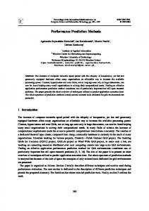
Fig. 1. Fine grained regression for workload throughput prediction on Amazon Web Services instances using TPC-DS.
All other progress indicator research only estimates query progress in terms of unit-less percentages. Query Performance Prediction In [14], [15] the researchers used machine learning to predict latency for analytical queries executing in isolation. In [16] the authors addressed the problem of query execution time prediction by using a white-box approach, namely by leveraging the detailed query plan and the corresponding cost model obtained from the query optimizer. In [9], [19] the authors built models of query interactions to predict the end-to-end latencies of batches of analytical queries. [12] used machine learning to predict query performance as a range. [13] created finer-grained latency predictions for individual queries executing under concurrency. We depart from this work by considering workloads executing on changing hardware platforms. III. F INE G RAINED P ROFILING In the section, we demonstrate that a simple, query-at-a-time modeling approach poorly predicts throughput for portable databases. This finding underlines the need for a more general profiling solution. In this approach, we create a model for each platform based on aggregating over its member queries. Our goal is to see if by analyzing the resource requirements of individual queries in our workload, we could build a model to describe how they would perform as a collection. By summing up how the member queries used resources, we could quantify the total strain on our system. In theory this approach should be promising. We build a profile of each workload where we sum up the strain that the member queries would place on the system if executed in isolation. This should indicate the rate at which our workload can make progress and hence predict throughput. However we found that in practice this approach fails to capture the lower level interactions among our queries. We cannot model savings from beneficial relationships such as shared scans. We also fail to capture slowdown, such as two memory-intensive queries creating expensive thrashing in the buffer pool.
We start by profiling the query templates on three dimensions: memory, CPU and I/Os executed. We collect this data from database logs. We created a vector for each template with these three parameters, which capture the resource footprint for the query. To describe a workload, we summed up this 3-D vector over all templates in the workload. We then built a model using multivariate regression to learn the throughput of individual workloads. In our multivariate regression, the independent variables were the summed memory, I/O and CPU usage, and the dependent variable was the throughput for the whole workload on a given hardware configuration. We built one model per hardware platform. We experimented with the TPC-H and TPC-DS workloads detailed in Section VIII-A. We found that this approach worked reasonably well in TPC-H, with an average relative error of 23%. This is because the TPC-H benchmark uses a simple schema of just one fact table and few dimension tables. The opportunity for complex (i.e., negative) interactions are limited because all of the queries are sharing the same bottleneck. In contrast, under the same framework, the prediction quality for TPC-DS was very poor, with a mean relative error of 1307%, as shown in Figure 1. The errors are a result of very complex interactions among the queries. The database has skew, and includes seven fact tables and many more dimension tables. There are various degrees of data overlap among the queries. For this more complex dataset we regressed to the mean. In other words, there was no clear correlation between this linear combination of variables and the throughput. Hence our models had very large yintercepts and negligible slopes for our independent variables. For most cases this does adequately, albeit via over-fitting. For 80% of our samples, on average we get within 40% of the correct throughput. Our simple model creates an inaccurate representation of the workload as it fails to capture such richer interplay among queries. This corroborates the findings in [13], [14].
Cloud& Provider& 2&
Sample&training&workloads&& locally&and&in&the&cloud&
1&
QpM&
Cloud& Provider& 1&
3& Model building Performance&& Predic;ons&
Sample&new& workloads& locally&
2&
Fig. 2.
Cloud& workload& 1& 4&
Incrementally&improve&the&& predic;ons&by&incorpora;ng&feedback&& from&the&cloud&
System for modeling and predicting workload throughput.
is part of the workload fingerprint, characterizes how the workload responds to changing I/O, CPU and memory availability. We explore the details of this sampling approach more in the proceeding sections. In addition, we evaluate each of our reference workloads in the cloud. Our framework seamlessly considers multiple cloud providers, regarding each cloud offering as a distinct hardware platform. By quantifying how these remote response surfaces varied, we determined common behavioral patterns for analytical workloads in the cloud. We learn from our reference workloads’ performance in the cloud rather than interpolating within the local testbed. This learning approach makes our framework robust to hardware platforms that exceed our local capacity. Next we sample new workloads that are disjoint from the training set. We locally simulate a representative set of hardware configurations for the new workloads, creating local response surface. Finally we create predictions for new workloads on remote platforms by comparing their response surface to that of the reference workloads. We present the details of this process in Section VI. In addition we incrementally improve our model for new workloads by adding in-cloud performance to its fingerprint. As we refine our fingerprint for the workload, we create higher quality predictions for new, unsampled platforms.
IV. P ORTABLE P REDICTION F RAMEWORK Our framework consists of several modules as outlined in Figure 2. First, we train our model using a variety of reference workloads, called training workloads. Next, we execute limited sampling on a new workload on the local testbed. After that we compare the new workload to the references and create a model for it. Finally, we leverage the model to create workload throughput predictions (i.e., Queries per Minute or QpM). Optionally we use a feedback loop to update our predictions as more execution samples become available from the new workloads. We initially sample the execution of our known workloads using the experimental configuration detailed in VIII-A. Essentially, a new workload consists of a collection of queries that the user would like to understand the performance of on different hardware configurations. We sample these workloads under many simulated hardware configurations and generate a three-dimensional local response surface. This surface, which
V. L OCAL R ESPONSE S URFACE C ONSTRUCTION In our design, we create a simple framework for simulating hardware configurations for each workload using a local testbed. When we evaluate our new queries locally we obviate the noisiness that may be caused by virtualization and multi-tenancy. Although we did not empirically find these complexities to be a significant factor, the local testbed allows us to control for them. We call our hardware simulation system a spoiler because it occupies resources that would otherwise be available to the workload.1 The spoiler manipulates resource availability on three dimensions: CPU time, I/O bandwidth and memory. We consider the local response surface to be an inexpensive surrogate for cloud performance. 1 We derive its name from the American colloquialism “something that is produced to compete with something else and make it less successful.”
VI. M ODEL B UILDING 7 6
QpM
5 4 3 2 1 2.5 16
2 14 1.5
12 10 1
CPU (GHz)
8 0.5
6 4
Memory (GB)
Fig. 3. Local response surface for a TPC-DS workload with high I/O availability. Responses are in queries per minute. Low I/O dimension not shown.
We experiment with a workload by slicing this three dimensional response surface along several planes. In doing so, we identify the resources upon which the workload is most reliant. Not surprisingly, the I/O bandwidth was the dominant factor in many cases, followed by the memory availability. We control the memory dimension by selectively taking away portions of our RAM. We did this by allocating the space in the spoiler and pinning it in memory. This forced the query to swap if it needed more than the available RAM. In our case we start with 4 gigabytes of memory and increment in steps of four until we reach our maximum of 16 gigabytes. We regulate the CPU dimension by taking a percent of the CPU to make available to the database. For simplicity we set our number of cores equal to our multiprogramming level (MPL). Hence each query had access to a single core. We simulated our system having access to 25%, 50%, 75% and 100% of the CPU time. We did this by making a top priority process that executes a large number of floating point operations. We time the duration of the arithmetic and sleep for the appropriate ratio of CPU time. We had a coarse-grained metric for I/O availability: low or high. Most cloud providers have few levels of quality of service for their I/O time. Some cloud service providers, such as Amazon Web Services, have started offering their users to provision I/Os per second as a premium option. We simulated this by making our high availability give the database unimpeded access to I/O bandwidth. For the low I/O bandwidth case we had a competing process that circularly scanned a very large file at equal priority to the workload. An example local response surface is depicted in Figure 3. We see that its throughput varies from one to seven QpM. This workload’s throughput exhibits a strong correlation with memory availability. Most contention was in the I/O subsystem both through scanning tables and through swapping intermediate results as memory becomes less plentiful.
We elected to use a prediction framework inspired by memory-based version of collaborative filtering [28] to model our workloads. This approach is typically used in recommender systems. In simplified terms, collaborative filtering identifies similar objects, compares them and makes predictions about their future behavior. This part of our framework is labelled as “model building” in Figure 2. One popular application for collaborative filtering is movie recommendations, which we shortly review as an analogous exercise. When a viewer v asks for a movie recommendation from a site such as Netflix, the service would first try to identify similar users. It would then average the scores that similar viewers had for movies that v has not seen yet to project ratings for v. It can then rank the projected ratings and return the top-k to v. In our case, we forecast QpM for a new workload. We compute the similarity for our new workload to that of our references. We then calculate a weighted average of their outcomes for the target cloud platform based on similarity. We found that by using these simple steps, we could achieve high quality predictions with little training on new workloads. Our implementation first normalizes each reference workload to make it comparable to others. We zero mean its throughputs and divide by the standard deviation. This enables us to account for different workloads having distinct scales in QpM. For each reference workload r and hardware configuration h, we have a throughput tr,h . We have an average throughput of ar and a standard deviation σr . We normalize each throughput as: tr,h =
tr,h − ar σr
This puts our throughputs on a scale of approximately -1...1. We apply this Gaussian normalization once per workload. This makes one workload comparable to the others. When we receive a new workload i, for which we are creating a prediction, we normalize it similarly and then compare it to all of our reference workloads. For i we have samples of it executing on a set of hardware configurations Hi . We discuss our sampling strategies in the next section. For each pair of workloads i, j we compute Si,j = Hi ∩ Hj or the hardware configurations on which both have executed. We can then estimate the similarity between i and j as: X 1 ti,h tj,h wi,j = |Si,j | h∈Si,j
The above weight wi,j approximates the Pearson similarity between the normalized performance of workload i and that of workload j. After that we forecast the workload’s QpM on a new hardware platform, h, by taking a similarity-based weighted average of their normalized throughputs: P j|S 6=∅,h∈Hj wi,j tj,h ti,h = P i,j j|Si,j 6=∅,h∈Hj |wi,j |
Query 1 2 3 4 5 Fig. 4.
1
2 X
3
4
5 &'#
X X
&(# &)#
X X
!"# !%#
!$# !"#
!$#
!%# !$#
!%#
!"# !%#
!"#
!$# !"#
!$#
!%# !%#
!$# !%#
!"#
*+,-#
An example of 2-D Latin hypercube sampling. Fig. 5. Example workload for throughput evaluation with three streams with a workload of a, b, and c.
This forecasting favors workloads that most closely resemble the one for which we are creating a prediction. We downplay those that are less relevant to our forecasts. Naturally we can only take this weighted average for the workloads that have trained on h, the platform we are modeling. We can create predictions for both local and incloud platforms using this technique. While we benefit if our local test bed physically has more resources than the cloud-based platforms upon which we predict, we can use the model for cloud platforms exceeding our local capabilities. The only requirement for us to create a prediction is that we have data capturing how training workloads respond to each remote platform. Experimentally we evaluate cloud platforms that are both greater and less than our local testbed in hardware capacity. We then derive the unnormalized throughput as: ti,h = ti,h σi + ai This is our final prediction. VII. S AMPLING We experimented with two sampling strategies for exploring a workload’s response surface. We first consider Latin hypercube sampling, a technique that randomly selects a subsection of the available space with predictable distributions. We also evaluate adaptive sampling, in which we recursively subdivide the space to characterize the novel parts of the response surface. Latin Hypercube Sampling Latin hypercube sampling is a popular way to characterize a surface by taking random samples from it. It was used in [13], [19] for a static hardware variant of this problem. It takes samples such that each plane in our space is intersected exactly once, as depicted in Figure 4. In the complete version of Figure 3, we first partition the response surface by I/O bandwidth, a dimension that has exactly two values for our configuration. We do this such that our dimensions are all of uniform size to adhere to the requirement that each plane is sampled exactly once. We then have two 4x4 planes and we sample each four times at random. Adaptive Sampling We submit that our local response surface is monotonic. This is intuitive; the more resources a workload has, the faster it will complete. To build a collaborative filtering model we need to determine its distribution of throughputs. Exhaustively evaluating this continuous surface is not practical. On average it would take us 88 hours to analyze a single workload if we did so in a coarse grid.
We also considered using a system such as [22], in which the authors explore a high dimensional surface of database configurations. They identify regions of uncertainty and sample the ones that are most likely to improve their model. However this technique is likely to evaluate more than is necessary because it presumes a non-monotonic surface. By exploiting the clear relationship between hardware capacity and performance, we may reduce our sampling requirements. Hence we propose an adaptive sampling of the space. We start by sampling the extreme points of our local response surface. This corresponds to (2.4 GHz, 16 GB, High) and (0.6 GHz,4 GB, Low) in the full version of Figure 3. We first test to see if the range established by these points is significant. If it is very small, then we stop. Otherwise we recursively subdivide the space until we have a well-defined model. We subdivide the space until we observe that the change in throughput is ≤n% of the response surface range. Our recursive exploration of the space first divides the response surface by I/O bandwidth. We do this because I/O bandwidth is the dimension most strongly correlated with throughput. After that we subdivide on memory availability. It too directly impacts the I/O bottleneck. Finally we sample among changing CPU resources if we have not reached a stopping condition. VIII. P RELIMINARY R ESULTS In this section, we first detail our experimental configurations. We then explore the cloud response surface, for which we are building our models. Next, we evaluate the effectiveness of our prediction framework for cloud performance based on complete sampling of the local response grid. After that, we investigate how our system performs with our two sampling strategies. Finally, we look at the efficacy of our models gaining feedback from cloud sampling. A. Experimental Configuration We experimented with TPC-DS and TPC-H, two popular analytical benchmarks at scale factor 10. We evaluated using all but the 5 longest running queries on TPC-H and using 74 of the 100 TPC-DS templates, again omitting the longest running ones. We did not use the TPC-DS templates that ran for greater than 5 minutes in isolation on our highest local hardware configuration. We elected to omit the longest running queries because under concurrency their execution times grow very rapidly and we kept the scope of our experiments to 24 hours or less each. Nonetheless a portion of our experiments
B. In Cloud Performance In Figure 6 we detail the throughput for our individual workloads as they are deployed on a variety of cloud instances. We see a monotonic surface much like the ones that we encounter with the local testbed. This indicates that there may be exploitable correlations between the two surfaces. For TPC-H we see that the majority of our workloads are of moderate intensity. They have a gradual increase in performance until they reach the extra large instance. At that point many of the workloads fit in the 7.5 GB of memory, seeing only modest gains from the largest instance. There are three workloads that are more intensive (shown in dashed lines). They have greater hardware requirements and do not see performance gains until the database is completely memory resident.
+"
#*"
*"
#("
)"
#&"
("
#$" !"#$%#&'(')%*"+#'
!"#$%#&'(')%*"+#'
(2%) still exhibited unbounded latency growth. We terminated them after 24 hours and record them as having zero QpM. We implemented a variant of the TPC-H throughput test. An example of our setup is displayed in Figure 5. Specifically we created a workload with 5 templates, ± 1 to account for modulus cases. Our trials were all at multiprogramming level 3, in accordance with TPC-H standards. Each of our three query streams executed a permutation of the workload’s templates. We executed at least 5 examples of each stream before we concluded our test. We omit the first and last few queries from each experiment to account for a warmup and cool down time. We compute the queries per minute (QpM) for the duration of the experiment. We created 23 TPC-DS workloads using this method. The first 8 were configured to look at increasing database sizes. The first two access tables totaling to 5 GB, the second two at 10 GB, et cetera. The remaining 15 workloads were randomly generated without replacement. For TPC-H we randomly generated 9 workloads. There were three sets of three permutations without replacement. We evaluate the quality of our predictions using mean relative error as in [13], [14], [19]. We compute it for each . This metric scales our preprediction as |observed−predicted| observed dictions by the throughputs, giving an intuitive yardstick for our errors. For our in-cloud evaluations we used Amazon EC2 and Rackspace. We rented EC2’s m1.medium, m1.large, m1.xlarge and hi1.4xlarge instances. The first three are general purpose virtual machines at increasing scale of hardware. The final is an I/O intensive SSD offering. We considered experimenting on their micro instances and conducted some experiments on AWS’s m1.small offering. However we found that so many of our workloads do not complete within our time requirement in this limited setting that we ceased pursuing this option. When a workload greatly outstrips the hardware resources available it is reduced to thrashing as it swaps continuously. In Rackspace we experimented on their 4, 8, 16, and 32 GB cloud offerings. We used k-fold cross validation (k=4) for all of our trials. That is, we partition our workloads into k equally sized folds, train on k − 1 folds and test on the remaining one.
'" &"
#!" *"
%"
("
$"
&"
#"
$"
!"
!" ,-./01"
Fig. 6.
2345-"
67345-"
8/59":;"
=?>"
8/59":;