First, the Harrod-. Domar growth model will lead to a hypothesis of one-way causality from financial development in economic growth. This is because, the ...
����������� ������� � ��������������
���������� � � � ��� ������������ �������������������������������������� � ����� ��� ���� ���� ��� ����� � � ���� ���� ���� ���������� ���� �� ������ �� �������� �� ��� � ������ �� � � ��� � ���� ������� ��� ��������� � ����� ���
��� � � ������! � � ��� ����� � �� ���� "���� ����� "�� �� �� ��� ���� � ���� ��
�������������� ������������ ��� �� ����� �� ����������������� ��� ������� ���� ������������� � ���#�������� ������� ��������� ���� "����
�������� � ��� �� ���
����������� �������
��������������������� ���
$� ���� ���"���� ��"� �� �$� �%� � ����&� ������ �������� ����������������� #���� ��&���� '�� � ���#�(�� ���$� ��� ����������� � ��� ������� )���� � �������*�� �� ������������� �� �+%( ���# &�)�)#��%,��� #�(�� ����#��)(&��� ���($)-.��/� �� ���"�� �������� ����! ���" � ��(� ��������
�� ������ ��/��� �/�������(� �� ����0�������1� �� ��"��
��� �� �
�����������������
�������� � ��� �� ��� �������������������������� � ����� �� �����������
�������� � ��� �� ���
�������������������������� � �� �� �� �����������
����������������� �������� ���
���������� ����� � � �������� �� ���� ��� �������������� ���� ���� �������� ������������� � � ���� �������� ��� ������ ���� ������ ������ ����� ��� ���� ����� �� � ���� ��������� ������� ����������������� �� ��� �������������������������
��������� �!�� ��� ��� � � � "���� ��� ������� �� � ��� ������ # ����� ���� �������� ���� ����������� $ ������ ��!%� � ����!� ����� � ������ ��� ��� & ���� ��$ � ���� ' ������ ��� ����� ������� ����� ' ������ ��� ���� (�$�������� �� ��� � ��� '������ ��� ���� # ����%� �������� ���%� )��� � �� ���%� * ������ ���% ' �������� �������� � $ �����������'�������� ����� � �� ������������ +������ ����� �� �� ��� ���� "�� ��%� � ��� ��� �� � ���� ��� &����� ��� ' ������ ��!�����# ����� ���������������� ��� ����������� ����$,��� ����� �������(����� �����������$��������� ��� �������� � � ��� ��� ����������� ����-�� ������� ��� ���� �������� ����. � ����� �� � ���� �������� ��� ������ � ��� ����� ����� ��� � �� ����� � � ���� ��������� ������� ������������� � � �� � � ��� � �� �������� ���������� �� ��������� �!�� �� � "�-��� ���� ���� �������� ��� ������������������ �������� ������(� ���� �� ��� ��%� �� ��� ��� � ����� ����� ����� ��� ��� �� ��� ���� ��� ���������� �� ��� ���� � � � ���� ����� ����� ������ � . �� ���� � � �� ��� � ���%� ����� � � ���%� ������� ���%��� ���� ���%������ ����� ����������� ������$�� ��� �� ��� �� ��� ���������� ���$�������������$ -������� �������������� ��� � �� � � ���� � -� ��� ��� ����� �� �������� ���� ��� ����� �� � � �� ��� ��� �� �� �������� ����������� ����� ��� ������ ������������-� �-��� /�����������/������� ����$$$ ����� �� �� 0��� ���������� ��� 1"��1"#�23.�" ���� ������� ��� ������������������������� ��� ��� ����
4���& �������)��*�5�/� �+) � � � ��� 6��78%�99:::�& ���� ���%������ � �����)��� �2� ������ �;����� ������ �� *��������������� ���������&������ �������� �������� ���� �� � ��������������������� ADF & KPSS (Critical values), it implies that unit root exist t* < ADF & KPSS (Critical values), it implies that unit root does not exist
For the ADF, the calculated statistics (t*) are those reported in Dickey-Fuller (1981).
The critical values at 1%, 5% and 10% are ±3.61, -2.94 and ±2.60.
For KPSS the critical values at 1%, 5% and 10% are 0.739, 0.463 and 0.347respectively (Kwiatkowski et al, 1992, table 1). 4.4 Testing for cointegration Testing for co-integration is relevant to the problem of determination of long-run
equilibrium
relationship.
Co-integration
is
the
statistical
implication of the existence of a long-run equilibrium relationship between variables. This step seeks to identify the number of cointegrating relationships that exist among these variables. This study uses the methodology developed by
79
Johansen (1991), popularly known as the Johansen cointegration test. The unit root test in table 4.2 satisfies the necessary condition for the usage of this test (uniform order of integration). This test identifies the number of stationary long-run relationships that exist among the set of integrated variables. It offers two tests, the trace test and the eigenvalue test, with a view to identifying the number of cointegrating relationships. Table 4.3 Results of Johansen Trace Statistics Test Null Alternative Trace Critical Hypothesis Statistics value 0.05 r=0 rt1 74.8687** 69.8189 rd1 rt2 53.6183** 47.8561 rd2 rt3 18.9146 29.7971 rd3 rt4 6.5091 15.4947 rd4 rt5 0.2434 3.8415
Prob**
0.0011 0.0151 0.4991 0.6353 0.6218
Trace test indicates 2 cointegration at the 0.05 level * denotes rejection of the hypothesis at the 0.05 level **MacKinnon-Haug-Michelis (1999) p-values
The trace test tests the null hypothesis that there are at most r cointegrating relationships. In other words, a rejection of the null hypothesis means that there are more than r cointegrating relationships. Table 4.3 displays the results from the trace test. The trace test rejects the null hypothesis if the trace statistics exceeds the critical value, which is generated automatically by Eviews. The first two rows of table 4.3 show that the trace statistics 74.8687 and 53.6183 exceed the critical values of 69.8189 and 47.8561
80
respectively at 95 percent confidence level. This suggests that the null hypothesis of no cointegrating relationships is rejected. This result confirms that there are two cointegrating relationships among the variables. Table 4.4 Results of Johansen Maximum Eigenvalue Critical Null Alternative ȿŵĂdž�ǀĂůƵĞ� value 0.05 Hypothesis r=0 r=1 42.2506** 33.8769 rd1 r=2 31.7037** 27.5843 rd2 r=3 12.4055 21.1316 rd3 r=4 6.2657 14.2646 rd4 r=5 0.2434 3.8415
Prob** 0.0001 0.0022 0.5082 0.5794 0.6218
Max-eigenvalue test indicates 2 cointegration at the 0.05 level * denotes rejection of the hypothesis at the 0.05 level **MacKinnon-Haug-Michelis (1999) p-values
The eigenvalue test tests the null hypothesis of r versus r+1 cointegrating relationships. This test rejects the null hypothesis if the eigenvalue test statistics exceeds the respective critical value. Table4.4 presents the results from this test. Similarly, the results from the first two rows of table 4.4 shows that, the eigenvalue test statistics, 42.2506 and 31.7037 exceed the critical values of 33.8769 and 27.5843 respectively, at 95 percent confidence level. This suggests that the null hypotheses be rejected. Hence, the failure to reject the alternative hypotheses indicate that there are two cointegrating relationship among the variables. These results confirm the presence of a long-run relationship between the explained variable and two of the explanatory variables.
81
The Long Run Model The result of the Johansen co-integration shows the existence of long run relationship among the variables. The co-integrating equation will be chosen based on log likelihood ratio. If the log likelihood ratio is positively signed, we chose the equation with the lowest log likelihood ratio and if negative signed, we chose the highest log likelihood ratio at absolute term. From the Johansen co-integration result, all the four log likelihood ratio of the respective co-integrating equations is positively signed. Therefore, the lowest log likelihood ratio is chosen. The lowest log likelihood ratio is 32.9505 and its corresponding co-integrating equation is stated below͖� RGDP = ± 14.2908 + 0.6091*M2/GDP + 0.2924*MCAP + 3.2546*IOP ± 0.0604*DR (0.1858)
(0.0250)
(0.53.12)
(0.0085)
Note: The Standard Error Statistics are those stated in parenthesis and * denotes that the parameters are significant in the long-run.
From the long run equation, if all independent variables are held constant, GDP will reduce by 14.2908 units in the long run. The coefficient of M2/GDP is +0.6091 implying a positive relationship between M2/GDP and GDP in the long run. A unit increase in M2/GDP will cause a rise in GDP by 0.6091units. The coefficient of MCAP is +0.2924. The coefficient is positively signed showing that in the long run, MCAP and RGDP are positively related. GDP
82
will increase in the long run by 0.2924units if MCAP increases by a unit. IOP has a coefficient of +3.2546. It can be deduced that in the long run, if IOP should increase by a unit; it will cause GDP to increase by 3.2546 units. The coefficient of DR is - 0.0604. The negatively signed coefficient signifies that DR and GDP have a negative long run relationship. A unit increase in DR means that GDP will decline by 0.0604units. All the variables except DR do not conform to the a priori expectations. This is because, deposit rate is a function of income and is positively related to income. The higher the income (per capital income), the higher the propensity to deposit part of the income not spent on consumption. 4.5 Vector Error Correction Following a thorough discussion of the cointegration results, the error correction model is estimated. There are at least three methods of estimating the error correction model. These include; Engle-Granger 2-step method, the Engle-Yoo, and the Johansen technique based on VAR. This study, however, chooses to use Engel-Granger 2-step method. The choice of this method is based on the fact that it is easy to use and possesses some unique capabilities. It is able to estimate both the short and long term effects of the explanatory variables on the explained variable as well as reporting the
83
various cointegrating equations. Also, it is able to determine the speed at which the explained variable returns to equilibrium after a deviation has occurred. 1. The error correction mechanism is the speed or degree of adjustment i.e. the rate at which the dependent variable adjust to changes in the independent variables. Since a long run equilibrium relationship has been established, the next step is test for the speed of adjustment using the short run dynamism of error correction mechanism (ECM). The ECM involves specifying an over-parameterized model (ECM-1) and afterwards, estimating a parsimonious model (ECM-2). Table 4.5 Result of the Over-Parametized Model (ECM-1) Dependent Variable D(RGDP-1) Variable Coefficient Std. Error t-Statistic Prob. D(RGDP) 0.356556 0.029904 2.435370 0.0182 D(M2/GDP-1) -2.021365 0.083828 -2.254868 0.0016 D(M2/GDP) -0.095847 0.070566 -1.358271 0.1903 D(IOP-1) 0.153104 0.191661 3.798827 0.0143 D(IOP) -0.324637 0.212901 -0.524827 0.2138 D(DR-1) -5.52E-05 0.004062 -0.013587 0.9893 D(DR) 0.542703 0.003985 5.678343 0.0057 D(MCAP) 0.002651 0.026543 0.099866 0.7615 D(MCAP-1) -0.013963 0.041169 -2.339165 0.0382 ECM-1 -0.215435 0.154556 -0.099866 0.9215 C -0.285745 1.456749 -0.196153 0.8466 R2 = 0.6774 Adjusted R2 = 6483 D.W = 1.334 AIC = 2.9667 SC = 2.5975
The over-parameterized ECM results above shows that the coefficient of the error correction term is significant with the negative sign. The ± sign
84
justifies its significance. This means that it will be effective to correct any deviations from the long-run equilibrium. The coefficient of ECM is 0.215435, indicating that, the speed of adjustment to long run equilibrium is 21.54% when any past deviation will be corrected in the present period. This implies that the present value of RGDP adjust slowly to changes in M2/GDP, MCAP, IOP, and DR. However, there is a need to simplify the model into a more interpretable and certainly more parsimonious model. The parsimonious model would be built by estimating the equations of only those variables found to be significant in the over-parameterized model. Table 4.6 Results of Parsimonious Model (ECM-2) Dependent Variable D(RGDP-1) Variable Coefficient Std. Error D(RGDP) D(M2/GDP-1) D(IOP-1) D(DR) D(MCAP-1) ECM-2 C
0.040367* 0.094182* 0.009178 -0.00232* 0.006295* -0.342200 -0.483713
t-Statistic
0.008535 4.729311 0.019634 4.796943 0.041952 0.218770 0.000614 -3.765416 0.011139 5.026473 0.073251 13.65171 0.103107 -4.691383
Prob. 0.0001 0.0001 0.8289 0.0011 0.0391 0.0010 0.0001
R2 = 0.9186 Adjusted R2 = 0.8914 D.W = 1.7668 AIC = -5.2877 SC = - 4.9105 EŽƚĞ͗�Ύ�ĚĞŶŽƚĞƐ�ƚŚĂƚ�ƚŚĞ�ĐŽĞĨĨŝĐŝĞŶƚƐ�ĂƌĞ�ƐŝŐŶŝĨŝĐĂŶƚ�Ăƚ�ϵϱй�ĐŽŶĨŝĚĞŶĐĞ�ůĞǀĞů͘� 6RXUFH��$XWKRU¶V�&RPSXWDWLRQ�
From the table above, it shows that the coefficient of ECM is -0.342200. The ECM is significant with the appropriate negative sign. The coefficient of the lagged ECM in the parsimonious model indicates that the speed of
85
adjustment of any past deviation to long run equilibrium is 34.2%. This shows that present value of the dependent variable adjust faster to changes in the independent variables than the 21.5% obtained in the over-parameterized model. The result of the parsimonious model also reveals that all variables except the lagged value of IOP is significant. Their significance was determined taking into consideration their probability value. The corresponding probability value of each variable must be less than 5%. It can be concluded that changes affecting RGDP are determined by M2/GDP, MCAP, DR in the short run and IOP in the long run. The table reveals that the coefficient of DR is negative while the coefficients of M2/GDP, MCAP and DR are positive. From the results, it could be deduced that M2/GDP has a direct relationship with RGDP because of the positively signed coefficient i.e. +0.09418. This implies that a unit increase in M2/GDP will lead to increase in RGDP by 0.09418 units. Also, the coefficient of IOP and RGDP are positively related. IOP has a coefficient of 0.006295. This means that if IOP should increase by a unit, RGDP will also increase by 0.006295 units. The results also indicate that MCAP and RGDP are positively related. The MCAP coefficient is +0.006295. A unit increase in MCAP will only cause RGDP to rise by 0.006295 units. However, the coefficient of DR (-0.002312) suggests that a negative
86
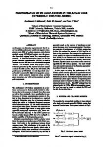
relationship subsists between DR and RGDP. The implication of a unit change in DR is that RGDP will consequently decrease by 0.002312 units. The coefficient of multiple determinations (R2) is 0.9186 and the adjusted value is 0.8914 which indicates that about 90% of total variation or a change in the present value of RGDP is explained by changes of past value in the explanatory variables while the remaining 10% is explained by other variation outside the model i.e. the error term. The Durbin Watson statistic of 1.7668 is indicative of the near absence of autocorrelation in the model. The residual graph of the parsimonious model which shows the actual and fitted observations is depicted below in Fig. 1. It indicates that the fitted observations are as close as possible to their observed value, which is the hallmark of Least Squares estimation. .15 .10 .05 .00
.03 .02
-.05
.01
-.10
.00 -.01 -.02 -.03 84
86
88
90
92
94
Residual
96
98
00
Actual
02
04
06
08
Fitted
Figure 4.6: Residua Graph of the Parsimonious Model
87
10
4.6
Vector Autoregressive (VAR) Model
Vector autoregressive (VAR) Model is an econometric
model used to
capture the linear interdependencies among multiple time series. VAR models generalize the univariate auto regression (AR) models by allowing for more than one evolving variable at more than one time period. In order to capture the feedback and dynamic relationships among macroeconomic variables of the model, the VAR model was used to estimate the response over time of any variables to the real gross domestic product RGDP). The VAR model establishes that real gross domestic product (RGDP) in Nigeria responds to shocks emanating from the financial sector. See appendix for the table. The results show that RGDP in the past years is positively related with the output in the first lag but becomes negative in the second lag. Financial deepening (M2/GDP) is positively related with the RGDP in both the first and second lags. Market Capitalization (MCAP) also is positively related to RGDP in both first and second lags. The index of openness (IOP) is negatively related to the RGDP in the first lag but becomes positive in the second lag. The rate of deposit (DR) also relates RGDP negatively in the first lag but becomes positive in the second lag.
88
Generally, the VAR results have corroborated both the long-run and shortrun equations of the cointegration and the Vector Error Correction model. 4.7 Causality Test
In order to ascertain the direction of causality among the variables, the study employed Pairwise Granger causality. The results of the test are presented in the table below: Table 4.7 Pairwise Granger Causality Tests Null Hypothesis:
Obs
F-Statistic
30
4.01172 3.92677
0.0146* 0.0042*
MCAP does not Granger Cause RGDP RGDP does not Granger Cause MCAP
30
1.78041 0.15396
0.1932 0.6979
IOP does not Granger Cause RGDP RGDP does not Granger Cause IOP
30
0.00151 2.86638
0.9693 0.1020
DR does not Granger Cause RGDP RGDP does not Granger Cause DR
30
0.15800 4.24554
0.6941 0.0256*
MCAP does not Granger Cause M2_GDP 30 M2_GDP does not Granger Cause MCAP
3.86341 4.93661
0.0310* 0.0114*
IOP does not Granger Cause M2_GDP M2_GDP does not Granger Cause IOP
30
0.24722 2.11171
0.6231 0.1577
DR does not Granger Cause M2_GDP M2_GDP does not Granger Cause DR
30
0.53113 0.07379
0.4724 0.7880
IOP does not Granger Cause MCAP MCAP does not Granger Cause IOP
30
5.01495 3.19012
0.0006* 0.0853
DR does not Granger Cause MCAP MCAP does not Granger Cause DR
30
3.70030 4.62541
0.0119* 0.0168*
DR does not Granger Cause IOP IOP does not Granger Cause DR
30
0.80649 0.33194
0.3771 0.5693
M2_GDP does not Granger Cause RGDP RGDP does not Granger Cause M2_GDP
89
Prob.
EŽƚĞ͗�Ύ�ĚĞŶŽƚĞƐ�ƌĞũĞĐƚŝŽŶ�ŽĨ�ƚŚĞ�ŶƵůů�ŚLJƉŽƚŚĞƐŝƐ�Ăƚ�ϱй�ƐŝŐŶŝĨŝĐĂŶĐĞ�ůĞǀĞů͘�� ZĞũĞĐƚŝŽŶ�ŽĨ�ƚŚĞ�ŶƵůů�ŚLJƉŽƚŚĞƐŝƐ�ŵĞĂŶƐ�ƚŚĂƚ�ĐĂƵƐĂůŝƚLJ�ĞdžŝƐƚƐ�ďĞƚǁĞĞŶ�ƚŚĞ�ǀĂƌŝĂďůĞƐ͘� 6RXUFH��$XWKRU¶V�&RPSXWDWLRQ�
Table 4.7 reveal bi-directional causation between financial deepening (M2/GDP) and real gross domestic product (RGDP) in Nigeria. That is, financial deepening causes GDP growth rate and real GDP on the other hand causes financial deepening, leading to the rejection of the null hypothesis of no causation. There is a unit-causation between real gross domestic product (RGDP) and deposit rate (DR) with causality proceeding from RGDP to DR. This conforms with a priori because, as the per capital income increases, chances are that, the rate at which people make deposits will increase giving that, savings is a function of income. Here too, the null hypothesis of no causation is rejected. The result of the granger causality test revealed a twoway causation between market capitalization (MCAP) and financial deepening (M2/GDP). This implies that, MCAP granger causes M2/GDP on one hand and M2/GDP granger cause MCAP. An increase in market capitalization is indicative of the level of development in the financial sector of the economy. Similarly, a developed financial sector is a catalyst for a robust capital market. A developed financial sector ensures investors
90
confidence in the capital market which ultimately lead to increased market capitalization. Thus, the null hypothesis of no causation between MCAP and M2/GDP is rejected. A unit-directional causation exists between index of openness (IOP) and market capitalization. This implies that, as the economy is open, foreign investments in the Nigerian capital market is encouraged. Foreigners buy shares on the Nigerian stock exchange and shares of Nigerian companies can as well be traded on the foreign exchanges. The null hypothesis of no causation between IOP and MCAP is therefore rejected. The granger causality results also revealed a two-way causation between market capitalization (MCAP) and deposit rate (DR). That is, MCAP granger causes DR on one hand and DR on the other hand granger cause MCAP. This implies that, as the market capitalization increases due to increase in deposits, more money is made available to
investors and
through the multiplier effect, the income of the people is enhanced thereby increasing the rate of deposit. Thus, the null hypothesis of no causality is rejected.
91
However, there is no sufficient statistical evidence to reject the null hypothesis of no causality between MCAP and RGDP, RGDP and MCAP; IOP and RGDP, RGDP and IOP; DR and RGDP; IOP and M2/GDP; MCAP and IOP; DR and IOP, IOP and DR at 5% level of significance. We therefore conclude that, there is no causation between these variables following the results of the granger causality test. Note that, the result of the granger causality test is independent of the cointegrating equation implying that, the estimates of the granger test are non-corroborative.
4.8 Impulse Response Function Impulse response functions trace the effect of a shock emanating from an endogenous variable to other variables in the VECM. It traces the long-run responses of the system variables to one standard deviation shocks to the system innovations spanning over the ten (10) quarters. The impulse response function for the model is analyzed below;
92
Res pons e of RGDP to Choles ky One S.D. Innovations
Res pons e of M2_GDP to Choles ky One S.D. Innovations
.06
.20 .15
.04 .10 .02
.05 .00
.00 -.05 -.02
-.10 1
2
3
4
5
RGDP IOP
6
7
M2_GDP DR
8
9
1
10
2
MCAP
3
4
5
RGDP IOP
Res pons e of MCAP to Choles ky One S.D. Innovations
6
7
M2_GDP DR
8
9
10
M CAP
Res pons e of IOP to Choles ky One S.D. Innovations
.3
.12
.2
.08
.1
.04
.0
.00
-.1
-.04
-.2
-.08 1
2
3
4
5
RGDP IOP
6
7
M2_GDP DR
8
9
1
10
MCAP
2
3
4
RGDP IOP
5
6
7
M2_GDP DR
Res pons e of DR to Choles ky One S.D. Innovations 4 3 2 1 0 -1 1
2
3
4
RGDP IOP
5
6 M2_GDP DR
7
8
9
10
MCAP
Figure 4.7: Combined Graphs of Impulse Response Function
93
8
9
M CAP
10
The result in figure 4.7 shows that each variable responds significantly to its own one-standard deviation shock. Furthermore, the results reveal RGDP responds to shocks in M2/GDP, MCAP, IOP, and DR (column 1, row 1). A one standard deviation shock to the innovations in M2/GDP would lead to a significant positive response in RGDP from the fourth quarter and then decrease consistently up to the tenth quarter horizon. A one standard deviation shock to MCAP would commence a moderate shock in the fourth quarter and rise smoothly up to the tenth quarter. Similarly, a one standard deviation shock to IOP would commence a shock in RGDP from the second quarter and it would decrease consistently up to the tenth quarter. Lastly, a shock to DR would commence in the second quarter and maintain a bowlike shape up to the tenth quarter. 4.9 Variance Decomposition Variance decompositions provide information about the relative importance of each random innovation in affecting the variables in the VECM. The results of variance decomposition of the model over a 10-quarter horizon are presented in Appendix 2. The variance decomposition apportions the total fluctuations in a particular variable to the constituent innovations in the system.
94
The results show that the variables are largely driven by themselves. For example, about 88.54 per cent of the variations in RGDP are due to its own innovations during the first quarter of the forecast horizon. The contribution M2/GDP alongside other variables to the variation in RGDP became significant in the 4th quarter with a combined total variation of about 24 percent. By the tenth quarter, the contribution of M2/GDP, MCAP, IOP and DR was 39.95, 3.24, 1.62 and 4.10 respectively. Thus, the principal drivers of RGDP are itself and M2/GDP. The variances of M2/GDP are driven primarily by itself in the first quarter, contributing about 91.18 percent, RGDP and DR contributing the remaining 8.82 percent of the total variations. By the second quarter, all the other variables collectively contribute about 11 per cent of the total variations in M2/GDP. RGDP emerges as the second major driver of M2/GDP, contributing about 20.13 percent of the total variations in M2/GDP by the end of the tenth quarter. The shares of MCAP and IOP in the total variations of M2/GDP stand at 4.96 and 2.23 per cent, respectively. The contribution of MCAP to variations in its own innovations stands at 87.30 percent in the first quarter. By the end of the 4th quarter, contribution of other variables to variations in MCAP accounted for nearly 40 percent of the total variations. RGDP contribution to the variations in MCAP stood at 31.23 percent by the
95
tenth quarter making it a major contributing variable to the variations in MCAP. With respect to variations in IOP, its own contribution stands at 89.30 per cent while RGDP, M2/GDP and MCAP jointly account for the remaining 10.70 percent variation during the first quarter of the forecast horizon. By the end of the 2nd quarter, the share of M2/GDP in total variation of IOP increased significantly to 31.75 per cent but decreased consistently up to the tenth quarter, giving way to DR to dominate in the tenth quarter contribution, accounting for 31.25 percent of the total variations. The variations in DR are largely driven by itself contributing 81.24 percent of the total variations in the first quarter of the forecast horizon. All other variables contribute significantly to the total variations as from the 2 nd quarter up to the end of the tenth quarter. However, the key variables driving DR are itself and RGDP. In sum, the variance decomposition shows that the significant variation for each variable is due largely to its own variations. Lastly, the results of variance decomposition analysis confirm the significant influence of the real gross domestic product (RGDP) and financial deepening (M2/GDP) on each other, suggesting that both financial sector development and output growth complement each other.
96
4.10 Test of Hypotheses Hypothesis 1 The null hypothesis of hypothesis 1of the study stated in chapter one as: ³Ho: Financial deepening does not granger causes economic growth or economic growth does not gUDQJH� FDXVH� ILQDQFLDO� GHHSHQLQJ´� was tested using the granger causality result presented in appendix 3. Decision Rule: Reject the null hypothesis if the probability value is less than the significance level (Prob. < D ). Decision: the probability value of no bi-causality between M2/GDP and RGDP (M2/GDP l RGDP) either way is 0.0146 and 0.0042 respectively. Taking a significance level of 5% which is approximately 0.05. Therefore, since the prob. values are all less than the significance level, we reject the null hypothesis and conclude that, there is a bi-directional causality between the financial deepening (M2/GDP) and real gross domestic product. Hypothesis II The null hypothesis of the second hypothesis of the study stated as; ³Ho: There is no significant casual relationship between financial GHHSHQLQJ� DQG� HFRQRPLF� JURZWK´� ZDV tested using both the long-run equation and the short-run equations.
97
For the long-run equation H0: b1 = 0 t* =
b1
G
=
0.6091 = 3.2783 0.1858
t0.025, 29 = 2.045 3.2783 > 2.045
Decision: Since t calculated (t*) is greater than t tabulated (t0.025, 29) at 5% level of significance, we reject the null hypothesis and conclude that, there is significant casual relationship between financial deepening and economic growth in the long run. For the short-run model The calculated t (t*) extracted from the parsimonious model is 4.796943 and the critical value of t (t0.025, 29) is 2.045. Decision: Since t*> t0.025,
29
(4.796943 > 2.045), we reject the null
hypothesis and conclude that, there is significant casual relationship between financial deepening and economic growth in the short-run. 4.11 Discussion of Findings The main aim of this study is to investigate the causal-effect relationship between financial deepening and economic growth in Nigeria over a period of 1981-2011. A vivid observation of the results shows that all the explanatory variables and their lagged variables are positively related to real
98
gross domestic product (RGDP) except deposit rate (DR) and its lagged value for both the long run and short run models. The implication of this is that, financial deepening among other explanatory variables used in the analysis are growth leading. In the short run and long run, financial deepening, market capitalization, index of openness exerted positive effects on economic growth. The positive and statistically significant effect of financial development is supportive of the supply leading hypothesis in accordance with the predictions by McKinnon (1973) and Shaw (1973). The results imply that financial development feeds economic growth through the channel of increased investment. In the short-run, deposit rate has a negative sign, suggesting that further financial sector reform measures need to be implemented to facilitate development of the sector for economic growth. The coefficient of the lagged error correction term (ECM-2) of the parsimonious model is negative and statistically significant, further confirming the existence of a long run relationship among real gross domestic product and its determinants. The magnitude of the coefficient implies that 34.2 percent of the disequilibrium FDXVHG� E\� SUHYLRXV� \HDU¶V� VKRFNV� FRQYHUJHV� EDFN� WR� WKH� ORQJ-run equilibrium in the current year. The regression results for the conditional ECM-2 of ǻRGDP show several desirable statistical features. The regression specification fits remarkably well and passes the diagnostic tests against
99
non-normal
residuals,
serial
autoregressive conditional
correlation,
heteroskedasticity,
heteroskedasticity at
the 5% level
and of
significance. The study finds evidence of bi-directional causality between financial deepening and economic growth in Nigeria as shown by the granger causality result. This implies that financial depth stimulates growth and, simultaneously, growth propels financial development. The expansion of the real sector can significantly influence development of the financial sector in Nigeria. Both the results of the impulse response function and the variance decomposition revealed that, all the real gross domestic product (RGDP) responds to its own shock and to shocks emanating other variables and that, variations in the variables are largely driven by themselves. For example, variations in real gross domestic product (RGDP) are driven primarily by its innovations in the first quarter, contributing about 88.54 percent of the total variations. Lastly, the results of variance decomposition analysis confirmed the significant influence of the real gross domestic product (RGDP) and financial deepening (M2/GDP) on each other, suggesting that both financial sector developments and output growth complement each other.
100
CHAPTER FIVE SUMMARY, CONCLUSION AND RECOMMENDATIONS 5.1 Summary The determination of the relationship between financial deepening and economic growth is significant in that development policies are implemented according to the direction of this relationship. It can be argued that supplyleading relationship may lead to financial sector liberalization policies. On the other hand, if the relationship is demand-following, more emphasis should be placed on other growth-enhancing policies. For this reason, this study empirically analysed the direction of causality between financial deepening and economic growth as well as the magnitude of the relationship in Nigeria over a period of thirty one years (1981-2011). The study is anchored on the Mckinnon±Shaw theory of financial liberalization which underscores the importance of the financial bottle-necks with regards to the depth of the financial sector and the growth of the economy. The data for the study was sourced from the various editions of the Central Bank statistical bulletins. The estimation process started with the examination of the stationarity property of the underlying time series data. The Augmented Dikker Fuller
101
(ADF) and KPSS Tests were used for testing for unit root. The estimated results confirmed that financial development, measured by the ratio of money supply to gross domestic product, market capitalization, index of openness, deposit rates, and economic growth proxy by real gross domestic product are non-stationary at the level but found stationary at the first differences. Hence, they are integrated of order one. We next examined the existence of cointegration among the stationary variables. The Johansen cointegration test was applied to examine the same. The estimated results declared that there is cointegration and hence, confirmed the existence of long run equilibrium relationship between financial development and economic growth. For the short run dynamics, the result of the vector error correction revealed a positive and significant relationship between financial deepening and economic growth. The coefficient of the parsimonious error correction term (ECM) of -0.34.2 indicated the speed at which the dependent variable adjusts to previous shocks in the explanatory variables. The Granger-causality test finally confirmed that finance development and economic growth are very interdependent in Nigeria during the period 19812011. There exists bi-directional causality between economic growth and financial deepening implying that, an enhanced economic growth is responsible for financial development in the economy. This is quite obvious
102
as with enhanced economic growth, the country opts for financial development. Hence, the dynamism of economic growth in the country will foster financial development and dynamism of financial development will faster economic growth in the economy. Also, impulse response function and variance decomposition tests were conducted to analyse the responses to each variable to its own shocks and shocks emanating from the associated variables. The result revealed that, each variable responded greater to its own shocks than shocks arising from other variables with the dependent variables responding to shocks of all the explanatory variables. The result of the variance decomposition revealed that, variations in all the variables are largely due to own innovations with financial deepening and economic growth complementing each other. 7KH�K\SRWKHVHV�RI�WKH�VWXG\�ZHUH�WHVWHG�XVLQJ�WKH�VWXGHQW¶V�W�WHVW�IRU�ERWK� the long-run and the short-run. The null hypothesis of both hypothesis I and II were rejected in favour of alternative implying that; (i)
Financial deepening granger causes economic and economic on the other hand granger cause financial deepening.
(ii)
There is significant causal relationship between financial deepening and economic growth.
103
5.Ϯ Conclusion In conclusion, the study examined the relationship between financial deepening and economic growth in Nigeria between 1981 and 2011. Following a detailed time series analysis, the findings revealed a bidirectional relationship between financial deepening and economic growth. The study also revealed that financial deepening has a positive and significant impact on economic growth in Nigeria. It provides an empirical basis for promoting financial development and economic growth. It has two important policy implications, especially for developing countries. First, to gain sustainable economic growth, it is desirable to further undertake financial reforms. Second, to take advantage of the positive interaction between financial and economic development, one should liberalize the economy while liberalizing the financial sector. In other words, strategies that promote development in the real economy should also be emphasized. 5.3
Recommendations
The study has underscored the importance of the financial sector in influencing economic growth in Nigeria. The findings indicate that economic growth can be stimulated by the adoption of both short run and long run policies that ensure development of the financial sector. The study therefore recommends the following;
104
i.
An enhancement of the financial sector policies (facilitation of the establishment of financial institutions; creating enabling legal environment for efficient allocation of credit to the private sector at reasonable rates, ensuring depositors safety) with a view of strengthening the sector for achieving output growth owing to its vital role in engendering economic growth.
ii.
The development of the financial sector is found to be demandleading, that is, as the economy grows, the demand for financial sector services increases thereby leading to its development. This study
therefore
recommends
that,
strengthening
other
determinants of economic growth such as increase in investment, human capital development, mechanization of the agricultural sector among others which indirectly affect financial deepening should be given priority for achieving both economic growth and financial development simultaneously. iii.
Based on the positive relationship that existed between economic growth and market capitalization in both the long run and short run, the study recommends strengthening of the operations of the Nigerian Stock Market, which serves as a source of medium and long term finance for investment. This is because, the robustness
105
of the market ensures investors confidence which ultimately leads to increase in the volume of transaction and consequently leads to the growth of the economy. iv.
The study also recommends the sustenance of the liberal foreign trade policy as it impacts positively on the economy. However, the export component of the economy needs be improved.
v.
The zero causation between economic growth and deposit rate implies a poor reward system that discourages savings, thereby leading to large volume of money outside of the bank and unaccounted for. The study therefore recommends that, the rates of interest on deposits should be reviewed upwards the same way it is constantly done on the cost of capital (lending rates) so as to achieve output growth through savings-investment relationship.
Limitations of the study All the independent variables used in the study indicate positive relationship with the dependent variable except deposit rate. This study therefore suggests that further studies should employ component analysis of the financial sector of the Nigerian economy with a view to having a better understanding of the inverse relationship between the deposit rate and the
106
economic growth. In addition, this study suggests the expansion of the model used above to accommodate more explanatory variables. The study has only examined the direction of causality and the relationship between financial development and economic growth in Nigeria. Any further research on this issue should consider the possibility of exploring the trickledown effect of a deepened financial sector.
107
References Abu-Bader, S. and Abu-Qarn, A., (2006) ³Financial development and economic growth nexu: Time series evidence from middle eastern and north African countries´, Munich Personal RePEc Archive (MPRA) Paper 972, University Library of Munich, Germany. Adelakun, O. J., (2011)�� ³Human Capital Development and Economic Growth in Nigeria ´. European Journal of Business and Management Vol. 3, no. 9, pp. 29-38 Adesoye, A. et al (2011) ³Monetary Policy and Financial Repression in Nigeria: Test of MacKinnon Hypothesis´. African Journal of Scientific Research Volume 5, no.1 $IDQJLGHK��8��-������ �³)LQDQFLDO�'HYHORSPHQW�DQG�$JULFXOWXUDO�,QYHVWPHQW� in Nigeria´. Journal of Economic and Management Sciences, 12(1), 11-27 $JX�� &�&�� DQG� -�2�� &KXNZX� ����� � ³7RGD� DQG�