Papers International Journal of Bifurcation and Chaos, Vol. 10, No. 4 (2000) 737–748 c World Scientific Publishing Company
CHAOS-BASED SIGNAL PROCESSING ´ DEDIEU∗ HERVE Department of Electrical Engineering, Swiss Federal Institute of Technology Lausanne, EL-Ecublens, CH-1015 Lausanne, Switzerland MACIEJ OGORZALEK† Department of Electrical Engineering, University of Mining and Metallurgy, al.Mickiewicza 30, 30-059 Krak´ ow, Poland Received June 2, 1999; Revised August 15, 1999 Given a time series measured (or generated) by a known or an unknown dynamical system we address a series of problems which can be considered as advanced signal processing tasks, namely: (1) section-wise approximation of the measured signal by pieces of trajectories from a chosen nonlinear dynamical system (model); (2) signal restoration when the measured signal has been corrupted e.g. by quantization; (3) signal coding and compression. These tasks can be addressed using a new approach to the shadowing problem based on nonlinear observability problem. Its goal is to reproduce initial conditions for a dynamical system under consideration (approximating waveform generator) giving rise to an orbit which is optimal in the sense of average distance from the measured (or prescribed) transient output waveform. We present the results obtained using the Chua’s circuit as approximating waveform generator.
1. Introduction
On the other hand, there is a definite need for advanced tools for nonlinear signal processing which could exploit a priori phenomenological knowledge. Nonlinear models can represent one of such tools when combined with other efficient methods. Our goal in this paper is to show that a nonlinear (possibly chaotic) deterministic model together with nonlinear control toolkit can be used to perform a variety of signal processing tasks such as:
An important problem in various applications consists of processing of data measured from a physical object/process or generated by a nonlinear dynamical system [Abarbanel, 1996; Kantz & Schreiber, 1997]. This is the case for example in observations taken in meteorology, seismic data, physiology, medical observations and measurements, measurements taken in electronic circuits or telecommunication channels just to name a few. Often it is possible to find mathematical models of such processes (in terms of equations describing their time evolution). Despite the effort furnished into the development of such models they were so far of little use for signal processing [Haykin & Principe, 1999]. ∗ †
• Section-wise approximation of the measured signal by pieces of trajectories from a chosen nonlinear dynamical system (model). Here we show that one can exploit: (1) models of the process under consideration; (2) appropriately chosen dynamical systems which do not necessarily reflect the properties of the considered system but in
E-mail:
[email protected] E-mail:
[email protected] 737
738 H. Dedieu & M. Ogorzalek
some sense can produce similar signals (in terms of dynamic range and spectrum). In experiments we confirm that Approximating Waveforms Generator (AWG) having “rich dynamics” in many cases give very good results of approximation. • Signal restoration. The signal approximation task is performed in such a way that we always obtain a trajectory which is best in the leastsquare sense and is a smooth trajectory produced by a deterministic nonlinear dynamical system. Such a method intrinsically has the capability of smoothing out the quantization effects. • Signal coding and compression. By nature of the two above described tasks we obtain a specific type of coding of sections of the measured signal by a series of initial condition points in the state space. Thus the signal can be compressed — instead of storing the whole waveform we can just store the model equations and a set of initial conditions which when applied to the model can regenerate (approximately) the measured trajectory. The main problem we will address and which constitutes the basis for all further developments is how to reproduce transient signals embedded in the dynamics of a chaotic oscillator by finding the underlying initial conditions at some initial time t0 of the transient. In our earlier work [Dedieu & Ogorzalek, 1994a, 1994b, 1995a, 1995b, 1995c] we proposed an adaptive algorithm to modify the initial conditions and a control strategy to force the successive outputs to converge to the target output signal. Although successful in many numerical experiments such a procedure had many disadvantages such as poor convergence properties, lack of solid theoretical base and lack of generality. This problem has been also addressed in the nonlinear dynamics literature as “shadowing” of chaotic trajectories although finding the initial condition was usually only a by-product of the shadowing procedure. In this paper we propose a better solution to this problem based on nonlinear observability concepts. We do not intend here to provide all answers for these problems. Having solved the base approximation problem (shadowing!) we would like to demonstrate by examples how powerful the proposed approach could be. Full details on each of the above-mentioned task will be given elsewhere.
2. Base Problem Statement Let us consider a continuous-time dynamical system S whose dynamics are governed by equations of the form (the so-called Lur’e systems [Vidyasagar, 1978]): ˙ x(t) = Ax(t) + Bu(t) y(t) = CT x(t)
(1)
u(t) = f [y(t)] where: x(t), B, C ∈ RN , y(t), u(t) ∈ R, A — N × N real matrix, f : R → R is a locally Lipschitz function for t ≥ 0. We will assume that the parameters of the system are chosen such that it operates in a chaotic mode. Now suppose that we observe a transient signal of finite length τf which is the output of the system S in a time interval [t0 , t0 + τf ]. Suppose that we do not have access to the state variables of S at any time. Let us suppose further that the trajectory associated with the signal {y(t)} begins with an initial state x0 = x(t0 ) and ends at a final state xf = x(t0 + τf ). Let us call T the orbit associated with the trajectory. Our problem is to find with maximum precision the initial conditions of the state variables of S − x0 on the basis of the observation of y(t) only, for t0 ≤ t ≤ t0 + τf , in order to be able to reproduce accurately the signal y(t) observed during the interval [t0 , t0 + τf ]. In control theory this problem is referred to as exact observability [Levine, 1996; Grabowski, 1999]. An effective solution to this problem could offer an efficient way for coding signals since we can imagine that S could be a chaotic oscillator with very rich dynamical behavior whose attractor embeds, for instance, trajectories produced by unknown biological oscillators (i.e. “E.C.G. oscillators”, “speech oscillators”). As an typical example we will show how the method works in the case of Chua’s oscillator.
3. Relation with Shadowing and Noise Reduction In the nonlinear dynamics literature closely related problems known as shadowing and noise removal have also been considered [Farmer & Sidorowich, 1991]. Let us briefly recall basic ideas.
Chaos-Based Signal Processing 739
Usually experimental measurement data are of discrete-time nature and we will assume in the sequel that we have a time series z(n) representing a scalar signal measured and stored from the process under consideration (e.g. samples of a signal transmitted through a communication channel or a measured ECG signal). We will assume that this measured signal consists of the signal of our interest y(n) (possibly information carrying) and a number of contaminating signals si (n): z(n) = y(n) + s1 (n) + s2 (n) + · · ·
(2)
To be able to distinguish our signal y(n) from the others we must find some individual characteristic of y(n) which the other signals si (n) or the measured signal z(n) does not possess. In practical problems one can distinguish two cases: 1. measurement noise (which we assume is also the case of distortion introduced by the transmission channel in telecommunications) — when the measured signal is corrupted by a contaminating noise: z(n) = y(n) + s(n) (3) 2. dynamic noise — when contaminating signals are already introduced in the system evolution: z(n + 1) = f [z(n)] + s(n)
(4)
In the first case, we consider a noise removal problem to reproduce the signal y(n) while in the second case we speak of so-called shadowing problem e.g. reproducing the exact (noise-free) trajectory of the purely deterministic system zk+1 = f (zk )
(5)
which stays close to yk (“shadows” yk ) Our problem as stated above can be considered as a shadowing problem. In the mathematics literature [Guckenheimer & Holmes, 1983] the emphasis is on the existence of the shadowing orbit provided we know a pseudo-orbit — an orbit where the points are independently perturbed at each successive iterate — like in the numerical iteration of maps when at each step or in physical measurements. A strong existence result is given by the shadowing lemma valid for hyperbolic flows (see e.g. [Guckenheimer & Holmes, 1983, p. 251]). We would like to stress also that reproduction of the initial condition is not directly the goal of shadowing.
There exist a number of algorithms for solving the shadowing and noise removal problems [Farmer & Sidorowich, 1991; Grassberger et al., 1993; Kantz & Schreiber, 1997]. Most of methods are based on optimization methods with constraints in the form of system equations. Unfortunately, such algorithms are not computationally efficient especially for long time series. Here we propose an alternative approach which proves to be very computationally efficient and applicable in several signal processing tasks.
4. Proposed Approach The output signal of the system 1 is given by: y(t) = CT eAt x0 + CT
Z
t
eA(t−τ ) Bf [y(τ )]dτ (6)
t0
Hence in a simplified form we can write: CT eAt x0 = y(t) − (g ∗ f )(t)
(7)
where g is the impulse response of the linear part of the system and ∗ denotes the convolution. Equation (7) is solvable iff y − g ∗ f belongs to the range of the observability map P : Rn 3 x0 −→ Px0 ∈ L2 (t0 , tk ), (Px0 )(t) = CT eAt x0
(8)
Let us assume for simplicity that all eigenvalues λk of A are simple. Then the system {ck etλk }nk=1 ⊂ L2 (t0 , tk ) spans the range of P (for the proof take subsequently the vectors of the standard Cartesian basis as x0 ). Here ck stands for the kth component of the vector C. Let G be the Gram matrix of this system and q be the vector of the scalar products (in L2 (t0 , tk )) of this system with the right-hand side of (7). Then using the orthogonal projection theorem one gets (9) Gx0 = q which can be solved giving the best least-square approximation of the initial point x0 .
5. Implementation of the Method For the implementation of the method without loss of generality we will assume in the sequel that t0 = 0.
740 H. Dedieu & M. Ogorzalek
We assume further that we have observed the output signal y(t) in some interval [0, Tf ]. Let Ts be a sampling period of the output signal such that we have stored its N + 1 samples (Tf = N Ts ). Sampling of the output signal obviously influences the quality of the obtained approximation. If Ts is small enough the integral in Eq. (6 ) can be approximated after sampling by a set of N + 1 equations k = 1, . . . , N + 1 of the form y(kTs ) = CT eAkTs x0 + CT g(kTs )
(10)
where g(kTs ) is an approximation of the integral in Eq. (6) evaluated at time kTs using the Simpson method, g(0) = 0. Let us define
every ∆t = 10−7 s). In all the experiments for approximation/initial condition reconstruction the signal has been downsampled by a factor of 50 i.e. every 50th point only in the time series has been considered for the approximation procedure. Let us show two simulation results when two chaotic sequences with different number of samples are used. In the first example for the horizon of 50 000 samples and for a precision close to the machine precision used for storing the initial condition, the reconstruction is almost perfect. The measured (original) signal and the reconstructed one 4 measured reconstructed
3
P (k) = C eAkTs T
and
T
z=
(11)
y(0) y(Ts ) − CT g(Ts ) .. .
2 1 0
(12)
−1
y(N Ts ) − CT g(N Ts )
−2
PT (0) .. .
−3
G=
T
(13)
−4 0
1
2
3
4
time
P (N ) Using the pseudo-inverse we obtain the following least-squares approximate formula for the initial condition (14) x0 = (GT G)−1 GT z The procedure which has been implemented in Matlab includes more realistic effects such as signal quantization, nonideality of elements and noise.
6. Processing of Signals Generated by a System with Known Model
5 4
x 10
Relative error (%) between the reconstructed signal and the original one 1.5
1
0.5
0
−0.5
−1
Let us consider now the problem of finding initial conditions for the chaotic Chua’s oscillator in order to reproduce a given waveform measured earlier from this system during a prescribed time τ . In order to perform the experiments we have generated by a computer program a long time series. We stored just one variable x1 — voltage across the C1 capacitor in Chua’s circuit. In the experiments, we used two sampled sequences with 50 000 samples, and 100 000 samples, respectively (sampled
−1.5 0
1
2
3 time
4
5 4
x 10
Fig. 1. Results of reconstruction when the sampled sequence contained 50 000 samples. The data and the initial condition are stored using floating point representation (maximum machine precision referred to later as “infinite precision”). The upper figure shows the comparison between the original signal and the reconstructed one. The lower figure shows the relative error between these two trajectories.
Chaos-Based Signal Processing 741 The measured (original) signal and the reconstructed one 4 measured reconstructed
3 2 1 0 −1 −2 −3 −4 0
2
4
6
8
time
10 4
x 10
Relative error (%) between the reconstructed signal and the original one 100 80 60 40 20 0 −20 −40 −60
Our simulations show that there exists a tradeoff between the length of the trajectory and the precision of the initial conditions. For a given precision in initial condition one cannot extend the length of the time series which provides an acceptable error of reconstruction beyond a certain limit (due to the effect of the sensitivity to initial condition). On the other hand, for a given trajectory length increasing the precision of the initial condition reduces the variance of reconstruction error. However increasing the precision of initial condition beyond a certain limit will not decrease the error variance; the reason is that there is an inherent lack of precision of initial state estimation (approximation of the integral in (6) and accumulation of the calculation errors act as a noise source) which results in eventual separation of the trajectory starting at this initial condition from the original one. Depending on the given or prescribed error tolerance, it would be necessary to make a statistical study of the error variance with respect to the trajectory length and the precision of the initial condition (e.g. 14, 16, 18 bit). As a rule of thumb for an error tolerance of 1% (relative error to the trajectory dynamical range) we choose to work with trajectory length of N = 50 000 and precision in initial conditions of 16 bit as acceptable levels.
−80 −100 0
2
4
6 time
8
10 4
x 10
Fig. 2. Results of reconstruction when the sampled sequence contained 100 000 samples. The upper figure shows the comparison between the original signal and the reconstructed one. The lower figure shows the relative error between these two trajectories.
When we extend the reconstruction horizon to 100 000 samples while maintaining the same precision for the initial condition it can be clearly noticed (Fig. 2) that the reconstruction fails — the effect of sensitivity to initial condition causes the trajectory to eventually diverge after staying close to the measured one in the initial interval. Figures 3 and 4 show the reconstruction error when the “time window” is 50 000 samples with the precision on the initial condition varying from 24 bit down to 8 bit. Comparing this error of reconstruction with that of Fig. 1, one can see that its dynamic range is decreased, especially in its final part.
6.1. Immunity to quantization errors We investigate in this section the ability of the reconstruction method to deal with the quantization effects introduced by the measurement channel. The method is restricted to systems whose equations of dynamics and parameters are known with good precision; although this framework could appear of little use at first sight, it is common in chaosbased communication applications to consider that the chaos-based receiver has full knowledge of the transmitter — this a priori knowledge is exploited to design nonlinear filters which have the capability to smooth the chaotic signal (carrier). As explained before, the aim of reconstruction is to find a true system trajectory close to the original one according to some least-squares criteria. For a reasonable horizon we have seen that the method tends to locate a true orbit which is in the vicinity of the original one. When quantization corrupts the measured trajectory the estimate (14) locates the initial point of a trajectory which is the closest to
742 H. Dedieu & M. Ogorzalek The measured (original) signal and the reconstructed one
Relative error (%) between the reconstructed signal and the original one 1.5
4 measured reconstructed
3
1
2 0.5
1 0
0
−1
−0.5
−2 −1
−3 −4 0
1
2
3
4
5
time
−1.5 0
1
2
x 10
The measured (original) signal and the reconstructed one
3
4
time
4
5 4
x 10
Relative error (%) between the reconstructed signal and the original one 4
4 measured reconstructed
3
3
2
2
1 1 0 0 −1 −1
−2
−2
−3 −4 0
1
2
3
4
time
5 4
x 10
−3 0
1
2
3 time
4
5 4
x 10
Fig. 3. Relative reconstruction error of when the sampled sequence contained 50 000 samples but when the precision on the initial condition changes from 24 bit (first row) to 16 bit (second row). Figures in the first column show comparison between the original and the reconstructed signal, and in the second column the relative error.
it in the least-squares sense. Figures 5 and 6 show the performances of the reconstruction process for six different quantization levels of y(t), i.e. 16, 12, 8, 6, 5 and 4 bits. One can see that even for the modest level of quantization of 5 bit the reconstruction process is efficient.
7. Processing of Signals Using Arbitrary Model In this section, we demonstrate that the approximation/reconstruction/coding tasks could be achieved even in cases when the model of the generating system is unknown. In such a case we try to use an
arbitrary model i.e. we approximate the measured signal interval by interval by pieces of trajectories of an arbitrarily chosen (chaotic) oscillator. We bear in mind only that the dynamic range of the oscillator should be similar to the dynamic range of the measured signal and possibly the frequency spectrum of the oscillator should cover the frequency spectrum of the signal. In the experiments we used the approximation method as described before but we introduced in the algorithm an upper limit for error introduced by approximation in the considered interval. Thus in the coding procedure we used an adaptive scheme for changing the approximation interval (horizon)
Chaos-Based Signal Processing 743 The measured (original) signal and the reconstructed one
Relative error (%) between the reconstructed signal and the original one 80
4 measured reconstructed
60
3
40
2
20
1
0 0 −20 −1
−40
−2
−60
−3 −4 0
−80 1
2
3
4
time
5
−100 0
1
2
x 10
The measured (original) signal and the reconstructed one
3
4
time
4
5 4
x 10
Relative error (%) between the reconstructed signal and the original one 80
4 measured reconstructed
60
3
40
2
20
1
0 0 −20 −1
−40
−2
−60
−3 −4 0
−80 1
2
3 time
4
5 4
x 10
−100 0
1
2
3
4
time
5 4
x 10
Fig. 4. Relative reconstruction error of reconstruction when the sampled sequence contained 50 000 samples but when the precision on the initial condition changes from 12 bit (the first row) down to 8 bit (the second row). Figures in the first column show comparison between the original and the reconstructed signal, and in the second column the relative error.
length. In order not to exceed the given error bounds the initial length of a considered interval was divided by two in the case the error bound has been exceeded and the reconstruction done once more for this smaller subinterval). Once the error bound was within the range for the considered interval the approximation procedure was restarted for the next (maximum length) interval which in turn could be subdivided using the power of 2 rule until error bounds were satisfied. In this way we obtained a sequence of initial conditions for each of the (possibly shortened) intervals and ensured that the approximation error satisfied the assumed upper bounds.
7.1. Approximation and coding of an artificially generated signal To make the first test we generated artificially 40 000 samples of a special kind of signal by a Matlab program. The signal was composed of square wave of amplitude 2.0 and frequency f0 = 500 Hz which was added with a sinusoidal signal of frequency f1 = 2400 Hz modulated by a saw-tooth waveform of frequency f0 . The combined signal was low-pass filtered by a first-order filter with a cut-off frequency of 4000 Hz. The obtained waveform can be seen in Fig. 7.
744 H. Dedieu & M. Ogorzalek
The reconstructed signal and the quantized and downsampled original 4
Relative error (%) between the reconstructed signal and the original one 1.5 error after reconstruction
measured, downsampled and quantized reconstructed
3
1
2
0.5
1 0 0 −0.5 −1 −1
−2
−1.5
−3 −4 0
1
2
3
4
time
5
−2 0
1
2
x 10
The reconstructed signal and the quantized and downsampled original 4
3
Relative error (%) between the reconstructed signal and the original one 2 error after reconstruction
3
1.5
2
1
1
0.5
0
0
−1
−0.5
−2
−1
−3
−1.5
1
2
3
4
time
5
−2 0
1
2
3
error after reconstruction
measured, downsampled and quantized reconstructed
3
2
2
1
1
0
0
−1
−1
−2
−2
−3
−3
2
3 time
5 4
x 10
Relative error (%) between the reconstructed signal and the original one 4
3
1
4
time
4
x 10
The reconstructed signal and the quantized and downsampled original 4
−4 0
5 4
x 10
measured, downsampled and quantized reconstructed
−4 0
4
time
4
4
5 4
x 10
−4 0
1
2
3 time
4
5 4
x 10
Fig. 5. Results of reconstruction for the sequence of 50 000 samples. The three rows of figures show the reconstruction behavior for three different quantization levels of y(t), 16 bit (top), 12 bit (middle) and 8 bit (bottom).
Chaos-Based Signal Processing 745
The reconstructed signal and the quantized and downsampled original 4
Relative error (%) between the reconstructed signal and the original one 2.5 error after reconstruction
measured, downsampled and quantized reconstructed
2
3
1.5 2 1 1
0.5
0
0 −0.5
−1
−1 −2 −1.5 −3 −4 0
−2 1
2
3
4
time
5
−2.5 0
1
2
x 10
The reconstructed signal and the quantized and downsampled original 4
3
Relative error (%) between the reconstructed signal and the original one 0.8 error after reconstruction
3
0.6
2
0.4
1
0.2
0
0
−1
−0.2
−2
−0.4
−3
−0.6
1
2
3
4
time
5 4
x 10
measured, downsampled and quantized reconstructed
−4 0
4
time
4
5
−0.8 0
1
2
The reconstructed signal and the quantized and downsampled original 4
3
4
time
4
x 10
5 4
x 10
Relative error (%) between the reconstructed signal and the original one 80 error after reconstruction
measured, downsampled and quantized reconstructed
60
3
40
2
20
1
0 0 −20 −1
−40
−2
−60
−3 −4 0
−80 1
2
3 time
4
5 4
x 10
−100 0
1
2
3 time
4
5 4
x 10
Fig. 6. Results of reconstruction for the sequence of 50 000 samples. The three rows of figures show the reconstruction behavior for three different quantization levels for y(t), 6 bit (top), 5 bit (middle) and 4 bit (bottom).
746 H. Dedieu & M. Ogorzalek 2.6
3
measured reconstructed 2.5
2
2.4
1 2.3
0 2.2
−1 2.1
−2
−3
2
1.9
0
2000
4000
6000
8000
10000
12000
14000
0
100
200
300
400
500
100
200
300
400
500
600
700
−3
0.08
8
0.06
x 10
6
4
0.04
2 0.02
0 0
−2 −0.02
−4
−6
−0.04
−8 −0.06
−10 −0.08
0
2000
4000
6000
8000
10000
12000
14000
−12
Fig. 7. Results of reconstruction of an arbitrarily generated signal. This signal is approximated by pieces of chaotic trajectories of Chua’s circuit. The maximum error has been fixed to 2.5% and precision of the initial conditions for each segment to 16 bit. Maximum interval length was set to 2048 iterates. The whole waveform could be stored and reconstructed using just 12 initial conditions! (We had to store 36 numbers representing initial conditions for 12 intervals.)
For generating approximating pieces of trajectories we used the standard Chua’s circuit (operating in the chaotic mode). The results obtained are truly astonishing — we obtained an excellent approximation of the signal which does not belong to the attractor of Chua’s circuit with pieces of chaotic trajectories. The maximum error has been fixed to 2.5% and precision of the initial conditions for each segment to 16 bit. Maximum interval length was set to 2048 iterates. The whole waveform could be stored and reconstructed using just 12 initial conditions! (We had to store 36 numbers representing initial conditions for 12 intervals.)
0
600
700
Fig. 8. Results of reconstruction of the ECG signal. This signal is approximated again by pieces of chaotic trajectories of Chua’s circuit. The approximation error has been fixed within 2.5% and the initial conditions for each segment are stored using 16 bit precision. The compression ratio in this case is of 8.76 (we need to store 45 parameters at 16 bit each (initial conditions for 15 intervals) + 15 times the lengths of the intervals coded at 9 bit).
7.2. Approximation and coding of an ECG signal To see how far one could push the usage of our method we tried some experiments with measured waveforms which seem totally uncorrelated with the waveforms of the Chua’s circuit — namely we tried to look if it were possible to approximate the real measured ECG signal by pieces of chaotic trajectories of Chua’s circuit. Entirely different from the artificially generated signal used before, the ECG waveform has very rapid transients and peaks which seem to preclude the possibility of approximation
Chaos-Based Signal Processing 747
using Chua’s circuit. However the results again prove the contrary! It should be noted however that some of the approximating pieces obtained belong to some remote areas of the chaotic attractor (not normally visited by trajectories except in special choices of initial conditions). In the experiment (Fig. 8) the error of approximation has been fixed within 2.5% and the initial conditions for each segment are stored using 16 bit precision. The compression ratio in this case is of 8.76 (we need to store 45 parameters at 16 bit each (initial conditions for 15 intervals) + 15 times the lengths of the intervals coded at 9 bit). Comparing the results obtained in terms of ECG compression ratios we stress here that our figures are still quite modest — typically state-ofthe-art ECG compression methods give results in the range of compression ratios 12–15 (at the 500 Hz sampling rate). One should however consider that our results have been obtained using “off the shelf oscillator”!! We expect much better results if an adequate model of the signal dynamics could be used.
8. Conclusions Nonlinear models with rich, possibly chaotic dynamics offer a potentially very useful tool to perform several advanced signal processing tasks. Combining the knowledge from nonlinear control theory together with nonlinear dynamics enabled us to propose some new algorithms. The approach is based on the new solution of shadowing problem using approaches known in the control literature to solve the nonlinear exact observability problem. Thus we are able to find the initial condition for a nonlinear system in order to reproduce in an optimal way a measured system output in a given time horizon. Solution of this problem given in solid mathematical terms opens new vistas for signal processing problems. Particular problems we considered in this paper are: 1. Signal approximation/reconstruction. 2. Signal coding and compression. The proposed approach for finding initial conditions as described in the paper can be performed recursively giving an excellent approximation of a given (measured) signal by sections of trajectories of a chosen model (waveform generator). One can impose bounds on the approximation error and the procedure will adapt the lengths of successive intervals accordingly in such a way that
the pieces of approximating trajectories starting from the initial conditions found for each of the intervals will be best in terms of least-squares error (always smaller then the bound). Astonishingly this approximation/reconstruction approach can be also used when no good model of system dynamics is known. Taking a “sufficiently rich” waveform generator (e.g. a suitable chaotic oscillator) we have shown that an arbitrary waveform could be approximated/reconstructed. Furthermore calculation of initial conditions for each interval offers an interesting possibility for signal coding and compression. The measured signal for which we performed section-wise chaotic (nonlinear) approximation using the described method is automatically coded by a set of points in the state space. The “code” consists of the generating model equations together with its parameters and a set of initial conditions and time interval lengths. At no additional computational cost we also obtain compression of the measured signal — instead of storing the whole waveform one can just store the “code”. Knowing the generating model and initial conditions one can easily regenerate the original signal. It should be stressed that the better fidelity of the model the better the results of reconstruction/approximation/compression. Currently among many problems which we continue to investigate are: model construction/identification using time series measurements; performance evaluation of the proposed approach for different kinds of input data (e.g. generated by high-order systems, hyperchaotic systems, nonhyperbolic systems, etc.); further investigation of the compression algorithm; smoothing and noise removal properties of the proposed algorithm; feature extraction capabilities of our approach.
Acknowledgment The authors would like to thank Prof. Piotr Grabowski for bringing to their attention the exact observability problem and detailed discussions.
References Abarbanel, H. D. I. [1996] Analysis of Observed Chaotic Data (Springer-Verlag, NY–Berlin–Heidelberg). Chen, G. & Dong, X. [1993] “From chaos to order — perspectives and methodologies in controlling chaotic nonlinear dynamical systems,” Int. J. Bifurcation and Chaos 3(6), 1363–1409.
748 H. Dedieu & M. Ogorzalek
Cox, S. M. & Roberts, A. J. [1995] “Initial conditions for models of dynamical systems,” Physica D85, 126–141. Dedieu, H. & Ogorzalek, M. J. [1994a] “Finding initial conditions of a chaotic oscillator in order to reproduce transient target signals,” Proc. NDES’94, Krak´ ow, pp. 123–128. Dedieu, H. & Ogorzalek, M. J. [1994b] “Controlling chaos in Chua’s circuit via sampled inputs,” Int. J. Bifurcation and Chaos 4(2), 447–455. Dedieu, H. & Ogorzalek, M. J. [1995a] “Identification and control of nonlinear dynamics for signal coding and compression,” Proc. European Conf. Circuit Theory and Design, Istanbul, Vol. 2, pp. 1137–1140. Dedieu, H. & Ogorzalek, M. J. [1995b] “Signal coding and compression based on chaos control techniques,” Proc. 1995 IEEE Int. Symp. Circuits and Systems, Seattle 2, pp. 1191–1194. Dedieu, H. & Ogorzalek, M. J. [1995c] “Identification and control of a particular class of chaotic systems,” SPIE Photonics East, Conf. ‘Chaotic Circuits for Communication’, Philadelphia, pp. 148–156. Farmer, J. D. & Sidorowich, J. J. [1991] “Optimal shadowing and noise reduction,” Physica Series D47, 373–392. Grabowski, P. [1999] Lecture Notes on Optimal Control Systems (AGH-UWN-D, Krakow, Poland).
Grassberger, P., Hegger, R., Kantz, H., Schaffrath, C. & Schreiber, T. [1993] “On noise reduction methods for chaotic data,” Chaos 3, 127–141. Guckenheimer, J. & Holmes, P. [1983] Nonlinear Oscillations, Dynamical Systems, and Bifurcations of Vector Fields (Springer-Verlag). Haykin, S. & Principe, J. [1999] “Making sense of a complex world,” IEEE Sign. Process. Mag. 15(3), 66–81. Judd, K. & Mees, A. [1995] “On selecting models for nonlinear time series,” Physica Series D82, 426–444. Kantz, H. & Schreiber, T. [1997] Nonlinear Time Series Analysis (Cambridge University Press). Levine, W. S. (ed.) [1996] “Observers,” The Control Handbook (CRC Press and IEEE Press), Chapter 37. Madan, R. (ed.) [1993] Chua’s Circuit: A Paradigm for Chaos, World Scientific Series on Nonlinear Science Series B (World Scientific, Singapore). Ogorzalek, M. J. [1993a] “Taming chaos: Part I — synchronisation,” IEEE Trans. Circuits Syst. CAS40(10), 693–699. Ogorzalek, M. J. [1993b] “Taming chaos: Part II — control,” IEEE Trans. Circuits Syst. CAS-40(10), 700–706. Vidyasagar, M. [1978] Nonlinear Systems Analysis (Prentice-Hall, Englewood Cliffs, NJ).