Parallel Banding Algorithm to Compute Exact ... - NUS Computing

Parallel Banding Algorithm to Compute Exact Distance Transform with the GPU ∗ Thanh-Tung Cao

Ke Tang

Anis Mohamed

Tiow-Seng Tan

School of Computing, National University of Singapore

Abstract We propose a Parallel Banding Algorithm (PBA) on the GPU to compute the exact Euclidean Distance Transform (EDT) for a binary image in 2D and higher dimensions. Partitioning the image into small bands to process and then merging them concurrently, PBA computes the exact EDT with optimal linear total work, high level of parallelism and a good memory access pattern. This work is the first attempt to exploit the enormous power of the GPU in computing the exact EDT, while prior works are only on approximation. Compared to these other algorithms in our experiments, our exact algorithm is still a few times faster in 2D and 3D for most input sizes. We illustrate the use of our algorithm in applications such as computing the Euclidean skeleton using the integer medial axis transform, performing morphological operations of 3D volumetric data, and constructing 2D weighted centroidal Voronoi diagrams. CR Categories: I.3.5 [Computer Graphics]: Computational Geometry and Object Modeling—Geometric algorithms; I.3.1 [Computer Graphics]: Hardware Architecture—Graphics processors Keywords: Computational geometry, Voronoi diagram, graphics hardware, stipple drawing, morphological operation.

1 Introduction Euclidean Distance Transform (EDT) is an important problem with a wide range of applications in image processing, computer vision, graphics and computational geometry [Cuisenaire 1999]. For a ddimensional grid with N = nd grid points where some S grid points are colored, or termed sites, and some (N −S) grid points are not colored (white), the EDT problem is to compute for each grid point the Euclidean distance from itself to the closest colored grid point, forming a so-called distance map. This problem is closely related to the Voronoi diagram computation where for each grid point we are interested in the actual closest colored grid point or site. Trivially, one can compute such a distance map sequentially in time O(S(N − S)). The two recent survey papers [Fabbri et al. 2008; Jones et al. 2006] compare and contrast many state-of-the-art sequential approaches to solving the problems in 2D and 3D, targeting mainly the exact EDT computation. One highlight there is that the exact EDT can be computed in linear time using a dimensionality reduction approach (see [Maurer et al. 2003]). For certain ap∗ Project webpage: http://www.comp.nus.edu.sg/∼tants/pba.html. Emails: {caothanh | tangke | mohameda | tants}@comp.nus.edu.sg. The research is supported by the National University of Singapore under grant R-252-000-337-112.

Figure 1: The original grayscale image (left) to produce the stipple drawing (right) by using weighted centroidal Voronoi diagram.

plications such as constructing the Delaunay Triangulation from a discrete Voronoi diagram [Rong et al. 2008], the accuracy of the diagram is crucial to guarantee the correctness of the constructed triangulation. In another development, for some graphics applications, it is useful to quickly compute a good approximation of the EDT. This is the approximate EDT problem where the distance values computed at some grid points need not be 100% accurate. The recent development in the computational power of the graphics hardware has made such approximation possible at a very high speed; see, for example, [Rong and Tan 2006; Rong and Tan 2007; Schneider et al. 2009]. In a related problem, EDT is used in computing (weighted) centroidal Voronoi diagram (CVD), a special Voronoi diagram in which each site lies exactly at the centroid of its Voronoi region; see Figure 1 for an application of CVD. The CVD can be generated from any set of input sites using Lloyd’s iterative algorithm [1982]. In each iteration, the algorithm computes the Voronoi diagram, locating the centroid of each Voronoi region, and then moving each site to the centroid of its Voronoi region. There were several attempts in computing the centroids of all Voronoi regions using the GPU [Vasconcelos et al. 2008; Bollig 2009]; however, they all restrict the processing of each Voronoi region to a preset area around the corresponding Voronoi site. They thus do not work for nonuniform distribution of sites where each Voronoi region can possibly spread across the whole grid. There are two contributions in this paper: (1) An efficient parallel algorithm, termed Parallel Banding Algorithm (PBA), to compute the exact EDT using the GPU. Our algorithm is work optimal, while able to utilize effectively the power of the modern GPUs. The novelty comes from a careful partitioning of the input image into bands to allow concurrent computation, and an efficient merging of the sub-results through clever manipulation of doubly linked lists embedded on a 2D texture. The algorithm implemented in CUDA [NVIDIA 2009] outperforms all GPU-based approximate EDT algorithms in 2D and 3D. (2) A novel approach to compute a CVD efficiently and accurately, overcoming the deficiency of prior works that limit the area of each Voronoi region. Our novelty here is through exploiting important properties of the exact Voronoi diagram to store and sum the intermediate results when processing the Voronoi regions.

The rest of the paper is organized as follows. Section 2 outlines related works on computing EDT. Section 3 reviews some important properties for computing the exact EDT, which are utilized in our algorithm discussed in Section 4. Section 5 presents the performance comparison of PBA with other state-of-the-art algorithms in 2D and 3D. Section 6 illustrates applications such as CVD that can benefit from our fast and accurate algorithm. Finally, Section 7 concludes the paper with some limitations of our approach.

2

Related work

Exact and Approximation. Both the exact and approximate EDT can be sequentially computed in time linear to the number of grid points N = nd in d-dimension. Maurer et al. [2003] use dimensionality reduction and partial Voronoi diagram construction to compute the exact EDT for a binary image of arbitrary dimension. For each dimension, the EDT can be computed by using the EDT in the next lower dimension to construct the intersection of the Voronoi regions of the sites with each “row” of the image. On the other hand, most approximate EDT algorithms are based on Danielsson’s vector propagation method [Danielsson 1980]. This method stores a vector pointed to the candidate site for each grid point in the image. These vectors are then propagated using a structuring element called vector template. Multiple templates are swept in some certain fashions across the image. These algorithms can produce highly accurate EDT with just a small number of grid points with inaccurate distance values, and the absolute distance error is bounded. PRAM Solutions. To cater to the need of applications that require a throughput of millions of pixels per second, several parallel EDT algorithms have been proposed. Lee et al. [2003] use dimensionality reduction together with the theorem proven by Kolountzakis and Kutulakos [1992] to compute the exact EDT in O(log2 N ) time using O(N ) processors. Redefining the problem of finding the intersection of the Voronoi diagram with each row of the image as the problem of finding proximate sites (which can be optimally computed in O(log n) time using O( logn n ) processors [Hayashi et al. 1998]), one can compute the exact EDT in O(log n) time [Wang et al. 2001]. All the algorithms above are developed in the EREW PRAM model. Better time complexity algorithms for the more powerful CRCW PRAM model are known; see [Wang et al. 2001]. Our algorithm is inspired by Hayashi et al. [1998], but is much simpler and more practical to implement on modern graphics hardware.

error. Cuntz and Kolb [2007] propose an improvement to JFA by using a hierarchical approach to reduce the total work to O(N ). However, their method has a high error rate as it relies on downsampling the input image to reduce the total work, while a Voronoi diagram is usually very sensitive to any slight change in the positions of sites that are nearby. This limits its uses in practice. Schneider et al. [2009] modify Danielsson’s vector templates slightly to allow concurrent propagation for pixels in the same row or column. Their line sweeping algorithm, termed SKW, can be implemented on the GPU with linear total work complexity and the resulting distance map is close to exact. However, SKW has a high time complexity of O(n), and usually does not run faster than JFA. This is because it can only perform parallel propagation of pixels in one row at a time (in 2D problem). With a limited texture size due to the limited memory of the GPU (hardware and 32 bits architecture) and the need to have 104 threads or more in order to optimally utilize the processing power of the GPU [NVIDIA 2009], SKW under-utilizes the GPU. On the other hand, there has been no report in computing the exact EDT in the GPU using either the exact sequential algorithm or the above-mentioned exact PRAM algorithms. This is possibly because, in order to tap the superior memory bandwidth and computing power of the GPU, a special SIMD-like programming paradigm has to be employed. Those mentioned algorithms are much too complex to fit into such a paradigm effectively. In the next two sections, we discuss our proposed Parallel Banding Algorithm that is exact, work optimal and faster than all existing works. It is designed following the dimensionality reduction principle, with the idea of banding to increase the level of parallelism and the idea of using doubly linked lists embedded on a texture to facilitate the fast merging operation.

3 Exact Euclidean Distance Transform This section reviews the general approach to compute the exact EDT in a dimensionality reduction manner. The initial idea is proposed by Kolountzakis and Kutulakos [1992], and further extended by [Hayashi et al. 1998], [Lee et al. 2003], and [Maurer et al. 2003]. Our discussion is in the 2D case, i.e. we discuss the computation done in one dimension (for each row) and then in the second dimension (for each column). The same idea can easily be extended to higher dimensions by repeating the computation for each additional dimension.

Graphics Hardware Solutions. The early attempts to compute the approximate distance transform using the graphics hardware include the work of Hoff et al. [1999]. They render a right-angle cone for each site in the image to approximate the distance function, and use the depth-testing graphics hardware to obtain the distance map. Their method suffers from overdrawing and tessellation error. Sud et al. [2006] use a bilinear interpolation equation to compute the distance vector at any point on a polygon using the distance vectors of the polygon vertices. Their method can compute highly accurate distance maps for complex models, but its complexity is dependent on the number of sites in the image. As such, it is not suitable for problems with many sites.

Consider a 2D binary image of size N = n × n. We want to determine the intersection of each column i in the image and the Voronoi diagram of the sites. Let Si,j be the nearest site, among all sites in row j, of the pixel (i, j), and let Si = {Si,j | Si,j ̸= NULL, j = 0, 1, 2, . . . , n − 1} be the collection of such closest sites for all pixels in column i. Note that Si,j is NULL when there is no site in row j. Let Pi be the set of sites whose Voronoi regions intersect the pixels in column i. These sites are termed the proximate sites of column i. Among them, each pixel in column i needs to determine which is its closest site. To help improve the efficiency of this computation, the following three straightforward facts are utilized; refer to Figure 2.

Recent methods use the vector propagation approach to compute the approximate distance transform in the GPU. Rong and Tan [2006; 2007] present the Jump Flooding Algorithm (JFA) to compute the EDT in O(log n) time using O(N ) processors. Although JFA can easily exploit the tremendous computing power and memory bandwidth of the GPU, it has a suboptimal total work complexity of O(N log n), and thus sometimes incurs long actual running time. Though the work provides some insight into the (expected) low error rate, it does not provide a bound on the absolute distance

Following the convention in graphics, the upper left corner of the image has coordinate (0, 0) and lower right corner (n − 1, n − 1). We assume that the distances from any two sites to a grid point are different. In case of a tie, the distance from the site with the smaller coordinate is considered smaller. Fact 1. Consider column i and let b(i1 , j) and b′ (i2 , j) be two sites in row j. If |i1 − i| < |i2 − i|, then the Voronoi region of b′ cannot intersect column i. 

first propagate the information among the first and the last pixels of all bands using a parallel prefix approach on these 2m1 pixels. With this, the first and the last pixel of each band have the correct information, whereas other pixels inside a band can then obtain the correct closest sites by updating (if needed) their current information with that of the first and the last pixel of their band. This can be done in parallel in constant time using N threads. Figure 2: Illustration of the three facts of the exact EDT.

This fact means that for each column i, there can be at most one site along a row that can potentially be a proximate site, or basically, Pi ⊆ Si . As a result, |Pi | ≤ n. Fact 2. Consider column i and let a(i1 , j1 ), b(i2 , j2 ), c(i3 , j3 ) be any three sites with j1 < j2 < j3 . Let the intersection of the perpendicular bisector of a and b and column i be p(i, u), and that of b and c be q(i, v). If u > v then the Voronoi region of b cannot intersect column i.  When the mentioned situation happens, we say that a and c dominate b on column i. In this case, b ∈ / Pi . Fact 3. Let q(i, v) and p(i, u) be two pixels in column i such that u > v, and let a(i1 , j1 ) and c(i3 , j3 ) be the closest sites to q and p respectively. Then we have j1 ≤ j3 .  This fact means that the proximate sites of column i have their Voronoi regions appear in exactly the same order as when they are sorted by their y-coordinates. With the above facts, the exact EDT computation is done by the following three phases: Phase 1: For each pixel (i, j), compute Si,j . Phase 2: Compute the set Pi for each column i using Si . Phase 3: Compute the closest site for each pixel (i, j) using Pi .

4 Parallel Banding Algorithm In this section, we present our Parallel Banding Algorithm to perform the above-mentioned three phases on the GPU.

4.1 Phase 1 - Band Sweeping In this phase, for each row, we want to compute the 1D Voronoi diagram using only those sites in the same row. A trivial approach would be to use a two-pass sweeping (left to right and then right to left sweeping), similar to SKW [Schneider et al. 2009]. This, however, restricts the parallelism to only one thread per row, potentially under-utilizing the GPU. One could also use a 1D JFA [Rong and Tan 2007] with better utilization of the GPU at the cost of higher total work. Another possibility would be to use a method similar to the work efficient parallel prefix sum [Harris et al. 2007]. This approach is too complicated as compared to our following simple, yet work and time efficient approach. Our approach extends the na¨ıve two-pass sweeping approach, with the introduction of bands to effectively increase the level of parallelism. First, we divide the input image into m1 vertical bands of equal size, and use one thread to handle one row in each band, performing the left-right sweeps. Next, for one site to propagate its information to a different band (on the same row), it has to be the closest site to the first or the last pixel of its band. As such, to combine the result of different bands into the needed answer, we

4.2 Phase 2 - Hierarchical Merging This phase computes the proximate sites Pi for each column i, given Si . The sequential implementation to determine Pi is to sweep sites in Si from topmost to bottommost, while maintaining a stack of sites that are potentially proximate sites. When a new site c in Si is reached, we examine (using Fact 2) whether the site b at the top of the stack is dominated by c and the site a at the second top position in the stack. If so, b is popped out of the stack, and the process of examination repeats with a taking the place of b. Once this is done, c is pushed onto the stack, and the sweeping continue. At the end of the process, the stack contains Pi . However, this approach restricts the level of parallelism to one thread per column. To increase parallelism, we employ again the idea of banding. First, we divide the input image into m2 horizontal bands of equal size. Let B = {B1 , B2 , . . . , Bm2 } be the set of horizontal bands. For each column in each band Bk , we employ one thread to run the above algorithm to compute its proximate sites. Let PiB be the set of proximate sites of column i considering only the sites inside the band B. Then, the challenge is to merge the m2 resulting sets B Pi k from different bands of column i into Pi . To do this, for each column i, we perform a bottom up merging where two sets of results PiU and PiV of two consecutive bands U and V (with U above V ) are merged into one at each level, forming the result of a bigger band U ∪ V , till there is only one band left. To do this, we treat PiU as a stack with sites sorted, having the largest y-coordinate at the top of the stack, and consider each site in PiV in increasing y-coordinate. For each site c in PiV , we repeat the above-mentioned algorithm by removing each site at the top of the stack that is dominated by the site right below it in the stack and c; see Algorithm 1 for details. Algorithm 1 Merging PiU and PiV 1: 2: 3: 4: 5: 6: 7: 8: 9: 10: 11: 12: 13: 14: 15: 16: 17:

Stack ← PiU for c ∈ PiV in increasing y-coordinate do while Stack.size() ≥ 2 do Let b and a be the top and second top items in Stack if a and c dominate b then Stack.pop() else Break the while-loop end if end while Stack.push(c) if the two sites at the top of Stack are from PiV then Break the for-loop end if end for Join those sites not yet processed in PiV to those in Stack return Stack

This algorithm uses two important points to achieve linear total work (proven in Section 4.4). First, refer to Line 12. When there are two sites of PiV in the Stack, no subsequent popping is possible and we thus can break the for-loop at Line 13. This is because sites in PiV cannot dominate each other. Second, we can implement

O(N ) total work and O(log n) time. The propagation across bands using parallel prefix can be done in O(nm1 log m1 ) = O(N ) total work in O(log m1 ) = O(log n) time. The last update for each pixel within a band can trivially be done in O(N ) total work and O(1) time, yielding the total work and time complexity as claimed. 

Figure 3: The doubly linked lists embedded on a 2D texture.

In practice, there is a limit on the number of threads that can run concurrently on the GPU. Thus, an m1 smaller than that in the proof (as is used in our experiments) already can fully utilize the GPU without penalty in the actual running time. The added advantage of a smaller m1 is that the work in the propagation across bands is reduced. Fact 5. Phase 2 takes O(N ) total work.

PiU

PiV

the Stack, and as doubly linked lists so that Line 16 can be done in constant time without going through each site in PiV . The doubly linked lists are embedded onto a 2D texture, termed proximate texture; Figure 3 shows the upper part of the proximate texture where the red pixels store potential proximate sites when the processing reaches the green row during the proximate sites computation for each band. For each site Si,j being considered as a proximate site of column i, we store two pointers on the proximate texture at position (i, j): one pointing to the previous proximate site Si,j1 and the other to the next proximate site Si,j2 of column i. These pointers can simply be the indices j1 and j2 of the rows correspond to these proximate sites. The first and the last pixel of each resulting band are used to store the positions of the head and the tail of its doubly linked list.

4.3

Phase 3 - Block Coloring

Proof. The total work to compute the proximate set for each column of each band is obviously O(N ). The number of merging operations performed for each column is (m2 − 1), leading to a total number of n(m2 − 1) merging with the Algorithm 1. Consider the ℓ-th merging, and suppose Kℓ sites are popped in the merging. Then, the while-loop in Line 3 to Line 10 is executed exactly Kℓ times. Due to the breaking condition in Line 12, the for-loop in Line 2 to Line 15 can be executed no more than Kℓ + 2 times. Line 16 can be done in O(1) work since we use doubly linked lists. As such, the total work of the merging process is no more than: ( ) ∑ ∑ ∑ Kℓ + (Kℓ + 2) = 2 Kℓ + 2 n (m2 − 1) ℓ

ℓ

ℓ

Since ∑ we can remove at most a total of N sites in all the merging,  ℓ Kℓ is O(N ). Thus, the total work of Phase 2 is O(N ).

This phase uses the set Pi , whose sites are linked as a list in increasing y-coordinate, of each column i to compute the closest site for each pixel (i, j) in the order of j = 0, 1, . . . , n − 1. At each pixel p, we check the distance of p to the two sites a and b where a is at the front and b is just after a in the list. If a is closer, then a is the closest site to p, and the process is repeated for the pixel after p. If not, we can remove a from the list since it can no longer affect any other pixel from p onward (by Fact 3), and use b in place of a as the front of the list to compute the closest site to p.

The above fact means that the total work of Phase 2 is not much affected by the choice of m2 . By taking m2 all the way up to n, we can have the highest level of parallelism. However, the merging operation still has some overhead, while there is a limit in the level of parallelism of a GPU in practice. By allowing flexible choice of the number of bands, we can tune the algorithm to work best on different GPUs.

One might attempt a parallel approach by using a thread to handle a segment of pixels in column i having the same closest site in order to increase the level of parallelism. Such an approach, however, yields a completely random pattern of write operations, and does not have good performance in practice for the current GPU.

Proof. The number of attempts needed for each block to confirm its closest sites is the number of Voronoi regions that intersect that block. In the worst case, this number can be m3 , causing the complexity to be O(m3 N ). 

Instead, we propose to color a block of m3 consecutive pixels in column i at a time, using m3 threads. Each thread looks at two sites a and b in the front of the list. In the first case, when its pixel already has a site nearer to a and b, it does nothing. In the second case, when its pixel is nearer to a than to b, then that thread sets the closest site to its pixel as a. Otherwise, in the third case, the thread advances the front of the list to b. The process is repeated until the thread handling the last pixel in the block does not advance the front of the list. After finishing a block of m3 pixels, we move on to the next block of m3 pixels.

4.4

Complexity Analysis

We now analyze the complexity of our algorithm. We show that Phase 1 and Phase 2 are work efficient, while Phase 3 is also efficient in most situations. Fact 4. Phase 1 takes O(N ) total work and O(log n) time. Proof. Choose m1 to be

n . log n

Then, the left-right sweep takes

Fact 6. Phase 3 takes O(m3 N ) total work in the worst case.

Although the presence of m3 means a super-linear total work for our algorithm, we can maintain optimal total work if we set m3 to be a small number. In practice as we experience in our extensive experiments, a small m3 value is sufficient to achieve good performance for the algorithm.

4.5 3D and Higher Dimensions Our algorithm can be easily extended to 3D and higher dimensions. For example, in the 3D case with N = n3 pixels, having done the computation as in the 2D case for each plane where z = k for k = 0, 1, 2, . . . , n − 1, we need to finalize the closest sites for each “row” of pixels (a, b, k) where a and b are fixed and k ranges from 0 to (n − 1). This is achieved by applying Phase 2 and Phase 3 on each such “row”. The current graphics hardware limits a 3D image to 5123 . In order to compute the EDT for a bigger volume of n3 grid points, instead of computing the result for the whole image, we can perform the computation slice by slice as follows. Let Lk : z = k be a slice where k is an integer between 0 and n − 1. We first compute for

each of the n × n pixels (i, j, k) its closest site among all sites with the same i and j as their x- and y-coordinate. This is done by simply projecting all the sites onto Lk . Then, we can use Phase 2 and Phase 3 of our algorithm once to compute the result along the x-axis on Lk and then again along the y-axis on Lk , to obtain the EDT for Lk . This approach is useful for 3D applications that need the result for just one or several slices at any moment. In general, consider the d dimensional problem where the input size is N = nd . To simplify our discussion, we assume that in dimension d, the effort to compute distance from one voxel to another is constant, although in fact it is O(d). For such a high dimensional problem, our algorithm performs one pass of Phase 1 and (d − 1) passes of Phase 2 and Phase 3, each of which takes linear time, thus the total work is only O(dN ). In contrast, the approach of JFA needs to perform log n passes; in each, one voxel propagates its information to 3d other voxels, thus the total work of JFA is O(3d N log n). And, the approach of SKW needs to perform 2d sweepings; in each, one voxel propagates its information to 3d−1 other voxels. As such, the total work of SKW is O(d 3d−1 N ). Therefore, when we increase d, the running time of JFA and SKW grows much faster than that of our algorithm.

5 Experiments All tests are run on an Intel Core2 Quad Q6600 2.4GHz CPU running Windows XP Professional SP3. The machine is equipped with 4GB DDR2 RAM. To be able to compare PBA implemented in CUDA with other state-of-the-art approaches, we implement JFA and SKW using CUDA as well. JFA is a simple algorithm and there is no issue for our implementation to achieve the same performance as that in [Rong and Tan 2006]. On the other hand, there are many implementation choices for SKW. [Schneider et al. 2009] uses nVidia 8800GTX graphics card in its performance studies; we verify that our implementation of SKW has a better performance than that of [Schneider et al. 2009] on the same graphics card before doing our comparison. In 2D cases, we run the experiments with nVidia GeForce GTX280 graphics card with 1GB of video RAM, whereas for 3D cases, we need nVidia Tesla C1060 graphics card (lower in performance than GTX280) for its large 4GB video RAM to run large enough experiments.

5.1 Parameters m1 , m2 and m3 The three parameters m1 , m2 and m3 are independent from each other, we can thus tune them independently to achieve the best per-

Figure 4: Percentage of running time of the different phases of PBA in 2D with optimized and unoptimized parameters.

Figure 5: Speedup of PBA using different number of bands for Phase 2.

formance on different GPUs. For our nVidia GTX280 graphics card, the best values to use are m1 = 16, m2 = 16 for all texture sizes, and m3 = 16, 8, 4, 2, 1 for texture sizes from 512 × 512 till 8192 × 8192. Using smaller m3 for bigger texture is better since the overhead is high when we use bigger m3 , while the benefit of having higher parallelism is lesser when the texture gets bigger. Figure 4 shows the improvement in running time with the best choice of our parameters, where the unoptimized case refers to having m1 = m2 = m3 = 1. The running time of the optimized case is normalized to the corresponding running time of the unoptimized case. This is to highlight the effect of the choices of parameters in the three phases of the algorithm. Notice that Phase 2 is the most time-consuming phase and the improvement with the idea of banding is very significant; Figure 5 shows the running time improvement to Phase 2 for different value of m2 . Notice that the larger the value of m2 , the better the performance of our algorithm until it encounters the overhead of merging.

5.2 Density of Sites The theoretical complexity of all the implemented algorithms are independent of the number of sites in the texture. However, the actual running time can be slightly affected, as shown in Figure 6 on a 1024×1024 texture. Our algorithm is slightly faster when there are very few sites, slower when 10% to 90% of the pixels are sites, and faster again when the number of sites increases further. This is probably because when the number of sites is so small, Phase 2 (which dominates the computational time) of our algorithm has very few sites to process, and the algorithm thus runs faster. On the other hand, when the percentage of sites is larger than 90%, many Voronoi regions intersect each column, thus fewer sites are removed during merging in Phase 2, and the algorithm is again faster. With this understanding, to have a fair comparison to other algorithms, we report results based on test cases with the density of sites set at slightly above 10% and locations of sites chosen randomly.

Figure 6: Performance of PBA on different densities of sites.

5.3

2D Running Time

(a)

(b)

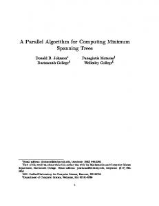
Figure 8: Speedup of PBA using optimal m1 , m2 and m3 , on different number of processors.

Figure 7: (a) 2D running time, and (b) normalized frame rates of different algorithms. Figure 7(a) presents the running time of different algorithms on different texture sizes ranging from 512 × 512 to 8192 × 8192. PBA performs significantly faster than all other algorithms, as it has a good balance of total work and level of parallelism to utilize the GPU. To appreciate the speedup of PBA better, Figure 7(b) shows the frame rates of different algorithms normalized to that of SKW. We use SKW as the baseline because it also has linear total work complexity. Our PBA performs up to 9 times faster than SKW on small texture sizes, but this ratio drops when the texture size increases. This is due to the limited number of processors of the GPU, when the texture is very big, SKW can also have enough level of parallelism to fully utilize the GPU. On the other hand, JFA is reasonably efficient for small size textures but performs the worst when texture size increases. For the largest texture, PBA outperforms JFA by a factor of 6 times. The above alludes to the fact that the advantage of PBA having a high level of parallelism diminishes for large texture sizes when compared to SKW. However, having a higher level of parallelism means that PBA scales better when the number of processors increases. To verify this claim, we use the NVStrap driver in the RivaTuner software to disable processing units in the nVidia 8800GTX card to generate Figure 8. It shows the speedup of PBA running on different numbers of stream processors (SPs), ranging from 16 to 128 (on the 8800GTX) and 240 (on the GTX280). Clearly, by choosing appropriate values for the parameters, PBA scales very well with the increase in the number of processors. The speedup is sub-linear because the memory bandwidth is unchanged (except from 128 SPs to 240 SPs). Note that historical evidence alludes to the fact that the increase in the number of stream processors is much faster than the increase in the support of larger textures. As such, we expect the performance of our new algorithm to continue to outperform all previous algorithms in the foreseeable future.

5.4

3D and Higher Dimensions

Figure 9(a) presents the running time of each algorithm. Clearly, our new algorithm outperforms all approximate EDT algorithms for most input sizes by a few times; see Figure 9(b). Figure 10 shows the breakdown on time for each phase of our algorithm, where the optimized cases use m1 = m3 = 1 and m2 = 2 or 4. The idea of banding plays a smaller role here in improving the performance of the algorithm as there is already enough level of parallelism (for current GPU) since we now have n2 rows of computation to be done concurrently in each of the three phases. Looking forward to the hardware that can support many more threads in the near future, our banding idea would remain advantageous. Also, as mentioned before, in case we need to compute EDT slice by slice for bigger volumes, the banding idea would be beneficial as the situation is similar to the 2D case.

(a)

(b)

Figure 9: (a) 3D running time, and (b) normalized frame rates of different algorithms.

Figure 10: Percentage of running time of the different phases of PBA in 3D with optimized and unoptimized parameters.

For the case of d > 4, due to the limitation on N , the size n of one dimension becomes very small (assuming a hypercube). One can trivially use Fact 1 to compute the exact EDT in O(nN ) total work. Since n is small, this algorithm achieves performance comparable to, if not better than, that of any above-mentioned algorithms due to its simplicity.

6 EDT Applications We illustrate the use of our fast exact EDT algorithm on a few applications in 2D and 3D.

6.1 Weighted Centroidal Voronoi Diagram Recall that the weighted centroid of a discrete Voronoi region is defined as: ∑ p∈V p w(p) Cs = ∑ s p∈Vs w(p)

Figure 11: Illustration of the weighted CVD computation.

where Vs is the Voronoi region of site s and w(p) is the weight of pixel p. We show how to compute the numerator, while the denominator can be computed in a similar way. Figure 11 shows one Voronoi region with the site at position (i, j) and notice that the region is not necessarily simply connected. A simple strategy is to sum up all the pixels horizontally first, and then add up these partial sums to obtain the final result. Note that Fact 3 states that pixels in one row belonging to the same site is connected, forming a chunk. Thus, if we can pre-compute the prefix sum for each pixel (i, j) along a row as:

Prefix(i, j) =

i−1 ∑

(a)

(b)

Figure 12: Performance of our weighted CVD computation on (a) different densities of sites and (b) different texture sizes.

6.2 Integer Medial Axis Given an exact EDT, Hesselink and Roerdink [2008] compute the Euclidean skeletons in linear time using the integer medial axis transform. Figure 13 shows some examples of such a skeleton on a 1024×1024 image, being generated at more than 300 frames per second. This allows real-time adjustment of various pruning parameters (such as γ) in the algorithm.

pk,j w(pk,j )

k=0

where pk,j is the pixel at (k, j). Then, knowing the starting and ending of a chunk, we can compute the sum of the chunk. The challenge lies in where to store the sum of each chunk for subsequent summing up as the sum of a Voronoi region. This is discussed in the next two paragraphs. Fact 1 states that if there is a chunk of pixels in row k belonging to the Voronoi region of site S at (i, j), then S must be the closest site to (i, k) among all sites in column i. As such, we can store the sum of this chunk at position (i, k) in a texture, termed sum texture, as no other sites (in particular those in column i) would possibly need this same storage space. So, all the partial sums that belong to site S are stored in column i as in the red region shown in Figure 11. Once we have set up the sum texture (as discussed in the next paragraph), a segmented scan [Sengupta et al. 2007] of each column of the sum texture gives the sum for each Voronoi region. To arrive at the partial sums in the sum texture using CUDA, we have the following implementation. Each block of threads is used to process a row. For block k processing row k, we use a shared array Arrayk of n elements. Each thread processing a pixel (ℓ, k) in the row k decides whether it is the leftmost pixel of a chunk belonging to a site (i, j). If yes, it stores Prefix(ℓ, k) in Arrayk [i]. Next, after synchronizing all threads, each thread processing a pixel (ℓ, k) in a row k decides whether it is the rightmost pixel of a chunk belonging to a site (i, j). If yes, it gets Prefix(ℓ + 1, k), subtracts the prefix sum stored in Arrayk [i], and stores the resulting sum of that chunk back to Arrayk [i]. Next, again after synchronizing all threads in the block, we write Arrayk into row k of the sum texture to complete the setup of the sum texture. The running time of the algorithm is almost independent of the density of the sites, with the exception that when the number of sites is very small the algorithm runs faster; see Figure 12(a). Figure 12(b) shows that our centroid computation algorithm scales linearly for different texture sizes. A direct application of our CVD algorithm is to create an artistic stipple drawing [Secord 2002]; see Figure 1. For such an application, there can be a large blank area without any sites, thus the Voronoi regions of sites on the boundary of this blank area can be elongated and become challenging cases to other existing works of CVD computation using the GPU.

(a) γ = 5

(b) γ = 10

(c) γ = 20

Figure 13: Euclidean skeletons of a binary image generated using integer medial axis transform.

6.3 Mathematical Morphology Morphological operators are very important in the processing of 3D volumetric data. The closing operation, which is a dilation followed by an erosion, can help removing cracks on a scanned model. The closing operation can be computed by performing EDT computation twice on the data set, one for computing the dilation, and one for the erosion. Figure 14 shows the closing operation applied on the UNC CThead 3D dataset of size 2563 . Using our exact EDT algorithm on the GPU, these images can be computed accurately and rendered at 5 to 6 frames per second, allowing interactive modification of the ball radius used by the operation. Note that other approximate EDT algorithms can achieve at most 2 to 3 frames per second.

Figure 14: The UNC CThead data set (leftmost) and its 3D distance closure of 5 voxels (middle) and 10 voxels (rightmost).

7

Conclusion

This paper presents the first efficient parallel algorithm on the GPU to compute the exact Euclidean distance transform (EDT) for binary images in 2D and higher dimensions. The algorithm is work efficient with linear total work, and with very high level of parallelism, allowing it to better utilize the enormous power of the GPU. Experiment results show that our exact algorithm still performs significantly faster than all known approximate EDT computation on the GPU. Importantly, our new algorithm scales well with the number of processors in the GPU, so it should work even better in the forthcoming generations of graphics cards with even larger number of processors. In addition to PBA, we present a weighted CVD algorithm that can accurately compute the centroids of all Voronoi regions in the GPU, independent of the number of regions and the size of each region. On the other hand, our Parallel Banding Algorithm still has some limitations. First, the merging workload for different threads in Phase 2 may not necessarily be balanced. It is possible that the merging pass of two sets of proximate sites can take up to O(n) time. In practice, this scenario hardly happens as it is almost impossible to produce a test case where the work loads on many columns of the image are unbalanced. Second, Phase 3 in the worst case (with large m3 ) is of non-optimal total work. One possible thinking is to break the set of proximate sites for each column into several subsets to be processed independently. Still, balancing the workload in such an approach remains challenging.

References B OLLIG , E. F. 2009. Centroidal Voronoi tesselation of manifolds using the GPU. Master’s thesis, Department of Scientific Computing, Florida State University. C UISENAIRE , O. 1999. Distance transformations: fast algorithms and applications to medical image processing. PhD thesis, Universite catholique de Louvain (UCL), Louvain-la-Neuve, Belgium. C UNTZ , N., AND KOLB , A. 2007. Fast hierarchical 3D distance transforms on the GPU. In Eurographics 2007, 93–96. DANIELSSON , P.-E. 1980. Euclidean distance mapping. Computer Graphics and Image Processing 14, 227–248. FABBRI , R., C OSTA , L. D. F., T ORELLI , J. C., AND B RUNO , O. M. 2008. 2D Euclidean distance transform algorithms: A comparative survey. ACM Computing Survey 40, 1, 1–44. H ARRIS , M., S ENGUPTA , S., AND OWENS , J. D. 2007. GPU Gems 3. Addison Wesley, ch. Parallel Prefix Sum (Scan) with CUDA, 815–876.

J ONES , M. W., BAERENTZEN , J. A., AND S RAMEK , M. 2006. 3D distance fields: A survey of techniques and applications. IEEE Transaction on Visualization and Computer Graphics 12, 4, 581–599. KOLOUNTZAKIS , M., AND K UTULAKOS , K. 1992. Fast computation of the Euclidean distance maps for binary images. Information Processing Letters 43, 181–184. L EE , Y.-H., H ORNG , S.-J., AND S EITZER , J. 2003. Parallel computation of the Euclidean distance transform on a threedimensional image array. IEEE Transaction on Parallel and Distributed Systems 14, 3, 203–212. L LOYD , S. W. 1982. Least square quantization in PCM. IEEE Transactions on Information Theory 28, 2, 129–137. M AURER , J R ., C. R., Q I , R., AND R AGHAVAN , V. 2003. A linear time algorithm for computing exact Euclidean distance transforms of binary images in arbitrary dimensions. IEEE Transactions on Pattern Analysis and Machine Intelligence 25, 2, 265– 270. NVIDIA. 2009. CUDA programming guide 2.0. RONG , G., AND TAN , T.-S. 2006. Jump flooding in GPU with applications to Voronoi diagram and distance transform. In I3D ’06: Proceedings of the 2006 symposium on Interactive 3D graphics and games, ACM, New York, NY, USA, 109–116. RONG , G., AND TAN , T.-S. 2007. Variants of jump flooding algorithm for computing discrete Voronoi diagrams. In ISVD ’07: Proceedings of the 4th International Symposium on Voronoi Diagrams in Science and Engineering, IEEE Computer Society, Washington, DC, USA, 176–181. RONG , G., TAN , T.-S., C AO , T.-T., AND S TEPHANUS. 2008. Computing two-dimensional Delaunay triangulation using graphics hardware. In I3D ’08: Proceedings of the 2008 Symposium on Interactive 3D Graphics and Games, ACM, New York, NY, USA, 89–97. S CHNEIDER , J., K RAUS , M., AND W ESTERMANN , R. 2009. GPU-based real-time discrete Euclidean distance transforms with precise error bounds. In International Conference on Computer Vision Theory and Applications (VISAPP), 435–442. S ECORD , A. 2002. Weighted Voronoi stippling. In NPAR ’02: Proceedings of the 2nd International Symposium on Nonphotorealistic Animation and Rendering, ACM, New York, NY, USA, 37–43. S ENGUPTA , S., H ARRIS , M., Z HANG , Y., AND OWENS , J. D. 2007. Scan primitives for GPU computing. In Graphics Hardware 2007, ACM, 97–106.

H AYASHI , T., NAKANO , K., AND O LARIU , S. 1998. Optimal parallel algorithms for finding proximate points, with applications. IEEE Transaction on Parallel and Distributed Systems 9, 12, 1153–1166.

S UD , A., G OVINDARAJU , N., G AYLE , R., AND M ANOCHA , D. 2006. Interactive 3D distance field computation using linear factorization. In I3D ’06: Proceedings of the 2006 Symposium on Interactive 3D Graphics and Games, ACM, New York, NY, USA, 117–124.

H ESSELINK , W., AND ROERDINK , J. 2008. Euclidean skeletons of digital image and volume data in linear time by the integer medial axis transform. IEEE Transactions on Pattern Analysis and Machine Intelligence 30, 12 (Dec.), 2204–2217.

VASCONCELOS , C. N., S A´ , A., C ARVALHO , P. C., AND G ATTASS , M. 2008. Lloyd’s algorithm on GPU. In ISVC ’08: Proceedings of the 4th International Symposium on Advances in Visual Computing, Springer-Verlag, Berlin, Heidelberg, 953–964.

H OFF , III, K. E., K EYSER , J., L IN , M., M ANOCHA , D., AND C ULVER , T. 1999. Fast computation of generalized Voronoi diagrams using graphics hardware. In SIGGRAPH ’99: Proceedings of the 26th Annual Conference on Computer Graphics and Interactive Techniques, 277–286.

WANG , Y.-R., H ORNG , S.-J., L EE , Y.-H., AND L EE , P.-Z. 2001. Optimal parallel algorithms for the 3D Euclidean distance transform on the CRCW and EREW PRAM models. Proc. of the 19th Workshop on Comb. Math. and Comp. Theory.