Chair, Supervisory Committee. Approved for the Major Department. Thomas C. Henderson. Chair/Dean. Approved for the Graduate Council. David S. Chapman.
PARALLEL COMPONENT INTERACTION WITH AN INTERFACE DEFINITION LANGUAGE COMPILER
by Kostadin Damevski
A thesis submitted to the faculty of The University of Utah in partial fulfillment of the requirements for the degree of
Master of Science in Computer Science
School of Computing The University of Utah May 2003
c Kostadin Damevski 2003 Copyright ° All Rights Reserved
THE UNIVERSITY OF UTAH GRADUATE SCHOOL
SUPERVISORY COMMITTEE APPROVAL
of a thesis submitted by
Kostadin Damevski
This thesis has been read by each member of the following supervisory committee and by majority vote has been found to be satisfactory.
Chair:
Steven G. Parker
Matthew Flatt
Gary E. Lindstrom
THE UNIVERSITY OF UTAH GRADUATE SCHOOL
FINAL READING APPROVAL
To the Graduate Council of the University of Utah:
in its final form and have I have read the thesis of Kostadin Damevski found that (1) its format, citations, and bibliographic style are consistent and acceptable; (2) its illustrative materials including figures, tables, and charts are in place; and (3) the final manuscript is satisfactory to the Supervisory Committee and is ready for submission to The Graduate School.
Date
Steven G. Parker Chair, Supervisory Committee
Approved for the Major Department
Thomas C. Henderson Chair/Dean
Approved for the Graduate Council
David S. Chapman Dean of The Graduate School
ABSTRACT Components can be a useful tool in software development, including the development of scientific computing applications. Many scientific applications require parallel execution, but commodity component models based on Remote Method Invocation (RMI) do not directly support the notion of parallel components. Parallel components raise questions about the semantics of method invocations and the mechanics of parallel data redistribution involving these components. Allowing parallel components to exist within a component framework comes at very little extra cost to the framework designer. However, the interaction semantics (i.e., method invocations) between two parallel components or between a parallel and nonparallel component can be complex and should require support from the underlying runtime system. The parallel data redistribution problem comes about when in order to increase efficiency, data are subdivided among cooperating parallel tasks within one component. When two or more components of this type are required to perform a separate computation on the same data, this data distribution must be decoded and mapped from the first component to the second component’s specification. We demonstrate a method to handle parallel method invocation and perform automatic data redistribution using the code generation process of an interface definition language (IDL) compiler. The generated code and runtime system accomplish the necessary data transfers and provide consistent behavior to method invocation. We describe the implementation of and semantics of Parallel Remote Method Invocation (PRMI). We describe how collective method calls can be used to provide coherent interactions between multiple components. Preliminary results and benchmarks are discussed.
CONTENTS ABSTRACT . . . . . . . . . . . . . . . . . . . . . . . . . . . . . . . . . . . . . . . . . . . . . . . . . . . . . .
iv
LIST OF FIGURES . . . . . . . . . . . . . . . . . . . . . . . . . . . . . . . . . . . . . . . . . . . . . . . vii LIST OF TABLES . . . . . . . . . . . . . . . . . . . . . . . . . . . . . . . . . . . . . . . . . . . . . . . . . viii ACKNOWLEDGEMENTS . . . . . . . . . . . . . . . . . . . . . . . . . . . . . . . . . . . . . . . . .
ix
CHAPTERS 1.
INTRODUCTION . . . . . . . . . . . . . . . . . . . . . . . . . . . . . . . . . . . . . . . . . . . . .
1
2.
COMPONENT FRAMEWORK TUTORIAL . . . . . . . . . . . . . . . . . . . . .
4
2.1 Components and IDL Basics . . . . . . . . . . . . . . . . . . . . . . . . . . . . . . . . . . . . 2.2 SCIRun2 Framework . . . . . . . . . . . . . . . . . . . . . . . . . . . . . . . . . . . . . . . . . .
4 6
3.
PRMI AND DATA REDISTRIBUTION SYSTEM OVERVIEW . . . 10 3.1 PRMI . . . . . . . . . . . . . . . . . . . . . . . . . . . . . . . . . . . . . . . . . . . . . . . . . . . . . 3.1.1 Collective . . . . . . . . . . . . . . . . . . . . . . . . . . . . . . . . . . . . . . . . . . . . . . 3.1.2 Independent . . . . . . . . . . . . . . . . . . . . . . . . . . . . . . . . . . . . . . . . . . . . 3.2 M-by-N Data Redistribution . . . . . . . . . . . . . . . . . . . . . . . . . . . . . . . . . . . .
4.
IMPLEMENTATION DETAILS . . . . . . . . . . . . . . . . . . . . . . . . . . . . . . . . 20 4.1 SIDL Compiler . . . . . . . . . . . . . . . . . . . . . . . . . . . . . . . . . . . . . . . . . . . . . . 4.2 PRMI . . . . . . . . . . . . . . . . . . . . . . . . . . . . . . . . . . . . . . . . . . . . . . . . . . . . . 4.2.1 Independent . . . . . . . . . . . . . . . . . . . . . . . . . . . . . . . . . . . . . . . . . . . . 4.2.2 Collective . . . . . . . . . . . . . . . . . . . . . . . . . . . . . . . . . . . . . . . . . . . . . . 4.3 M by N Data Redistribution . . . . . . . . . . . . . . . . . . . . . . . . . . . . . . . . . . . . 4.3.1 Overview . . . . . . . . . . . . . . . . . . . . . . . . . . . . . . . . . . . . . . . . . . . . . . . 4.3.2 Distribution Expression Methods . . . . . . . . . . . . . . . . . . . . . . . . . . . . 4.3.3 Runtime Objects . . . . . . . . . . . . . . . . . . . . . . . . . . . . . . . . . . . . . . . . . 4.3.4 Index Intersection . . . . . . . . . . . . . . . . . . . . . . . . . . . . . . . . . . . . . . . . 4.3.5 Data Transfer . . . . . . . . . . . . . . . . . . . . . . . . . . . . . . . . . . . . . . . . . . .
5.
10 11 14 14
20 22 23 24 26 26 27 29 29 31
RESULTS . . . . . . . . . . . . . . . . . . . . . . . . . . . . . . . . . . . . . . . . . . . . . . . . . . . . . 34 5.1 Choosing Characteristic Applications . . . . . . . . . . . . . . . . . . . . . . . . . . . . . 5.1.1 Jacobi Solution to the Laplace Heat Equation . . . . . . . . . . . . . . . . . . 5.1.2 LU Matrix Factorization . . . . . . . . . . . . . . . . . . . . . . . . . . . . . . . . . . . 5.1.3 Odd-Even Merge Sort . . . . . . . . . . . . . . . . . . . . . . . . . . . . . . . . . . . . . 5.2 System Scaling . . . . . . . . . . . . . . . . . . . . . . . . . . . . . . . . . . . . . . . . . . . . . . 5.3 Overhead Analysis . . . . . . . . . . . . . . . . . . . . . . . . . . . . . . . . . . . . . . . . . . . .
34 35 36 36 37 39
5.4 Comparison to Similar Systems . . . . . . . . . . . . . . . . . . . . . . . . . . . . . . . . . . 6.
41
CONCLUSIONS AND FUTURE RESEARCH . . . . . . . . . . . . . . . . . . . 43
APPENDICES A. SIDL INTERFACES TO EXAMPLE APPLICATIONS . . . . . . . . . . . . 45 B. SOURCE CODE TO ODD-EVEN MERGE SORT . . . . . . . . . . . . . . . . 47 REFERENCES . . . . . . . . . . . . . . . . . . . . . . . . . . . . . . . . . . . . . . . . . . . . . . . . . . . 54
vi
LIST OF FIGURES 2.1 A Remote Method Invocation (RMI) of two components. . . . . . . . . . . . . . .
5
2.2 A simulation performed using the original SCIRun framework.
.........
6
2.3 Elements of a CCA-compliant framework. . . . . . . . . . . . . . . . . . . . . . . . . . .
9
3.1 M = N collective PRMI diagram.
................................
12
3.2 M > N collective PRMI diagram.
................................
13
3.3 M < N collective PRMI diagram.
................................
14
3.4 Description of a distribution index. . . . . . . . . . . . . . . . . . . . . . . . . . . . . . . .
18
3.5 Example of a data redistribution pattern. . . . . . . . . . . . . . . . . . . . . . . . . . .
19
4.1 The input and output files of our SIDL compiler implementation. . . . . . . . .
21
4.2 Data transfer example. . . . . . . . . . . . . . . . . . . . . . . . . . . . . . . . . . . . . . . . . .
31
5.1 System scaling graph. . . . . . . . . . . . . . . . . . . . . . . . . . . . . . . . . . . . . . . . . . .
38
5.2 M-by-N overhead analysis. . . . . . . . . . . . . . . . . . . . . . . . . . . . . . . . . . . . . . . .
40
5.3 Comparison of LU Factorization performance of SCIRun2 and Global Arrays. 42
LIST OF TABLES 5.1 Jacobi’s algorithm running times using two parallel processes. . . . . . . . . . . .
37
5.2 LU Factorization algorithm running times using six parallel processes. . . . .
37
5.3 Odd-Even Sort running times using four parallel processes. . . . . . . . . . . . . .
38
5.4 Invocation comparison. . . . . . . . . . . . . . . . . . . . . . . . . . . . . . . . . . . . . . . . . .
40
5.5 Global Arrays comparison of LU Factorization algorithm running times using four parallel processes. . . . . . . . . . . . . . . . . . . . . . . . . . . . . . . . . . . . . .
41
ACKNOWLEDGEMENTS I would like to thank Dr. Steven Parker for developing the design upon which this thesis is based, as well as providing excellent guidance through the work. I would also like to thank Scott Owens for helping me develop a robust and efficient algorithm for the array slicing problem, and Jason Waltman for providing me with feedback on various versions of this manuscript. Thanks to the CCA group at the University of Utah for listening to my ideas and an atmosphere of collaboration. Finally, I would like to thank everyone who is close to me and supported me through my various struggles and days of self-doubt.
CHAPTER 1 INTRODUCTION The goal of this work is to propose a simple method to handle parallel method invocations and a way to build data redistribution on top of these invocations. One way of developing such a system is by utilizing the code generation process of an interface definition language (IDL) compiler to perform the necessary data manipulations and provide a consistent behavior in parallel component method invocations. This thesis will describe such a system; one that is reliant mainly on specifications provided at the interface level to provide the necessary data redistribution and limited to the case of multidimensional arrays. Component technology is an important and widely used tool in software development. However, commodity component implementations do not support the needs of high performance scientific computing.
To remedy this, the CCA (Common Component
Architecture) [1] group was formed among various universities and research institutions, including the University of Utah, Indiana University, Department of Energy research laboratories, and others. The group’s goal is to add the functionality of components to existing scientific computing code while preserving the natural speed and efficiency that this code contains. Parallelism is a tool that is consistently leveraged by many scientific programmers in order to increase performance. As a result, the ability to support parallel components is crucial when trying to provide components for scientific computing. The choice of parallel programming model for this purpose is SPMD (Single Program Multiple Data). Parallel components can be based on MPI (Message Passing Interface), PVM (Parallel Virtual Machine) or any other product that facilitates this very common type of parallel programming. Allowing parallel components to exist within a component framework comes at very little extra cost to the framework designer. However, the interaction semantics (i.e., method invocations) between two parallel components and between a parallel and nonparallel component is not clear and does require support from the com-
2 ponent framework. This is especially true when the number of processes differ between the caller and callee components. When we factor in the possibility of having distributed components, we use the term PRMI (Parallel Remote Method Invocation) to describe this type of a method invocation. Possible ways of defining PRMI can be seen in the work of Maasen et al. [15]; however there is no evidence to date of a definite decision on the specific semantics of PRMI. From a practical standpoint, a policy that will describe expected behavior when utilizing PRMI is required. M-by-N data redistribution is also an important piece of the high performance scientific components puzzle. The M-by-N problem comes about when, in order to increase efficiency, data are subdivided among M cooperating parallel tasks within one component. When two or more components of this type are required to perform a separate computation on the same data, this data distribution has to be decoded and mapped from the first component to the second component’s specification. Because each component can require a different data distribution to a separate number of parallel tasks, this problem can get complicated. Also, since components can be connected at runtime, their distribution requirements are not known a priori. Therefore, data transfer schedules have to be computed ad hoc. The M-by-N problem has been discussed among scientific computing researchers for a substantial period of time and systems such as PAWS [2], CUMULVS [8] and others have been developed that solve this problem for the limited case of multidimensional arrays. All of these systems are based on a specific data transfer API (Application Programming Interface). The data transfer API is separate from the actual method invocations. These systems have created a general solution to the M-by-N problem.
However, each of
them has taken a different approach to data representation and the timing, locking, and synchronization of the data transfer. The emergence of the CCA group has created a unique opportinuty to attempt to create a component framework standard for each of these issues. In addition, some of the M-by-N work suggests that in order to achieve maximum flexibility in the design, a specific M-by-N interface component needs to be in place [12]. This redistribution component will stand between two components that require a data distribution and perform this distribution for them. We recognize the added flexibility of this design; however we argue against it simply because of its inherent inefficiency. By choosing to base our M-by-N distribution mechanism on the PRMI, we decided to
3 treat the distribution data as another method argument in a PRMI invocation. Naturally, this choice led us to placing all of the necessary pieces to perform a data redistribution from M to N processes in the Interface Definition Language (IDL) compiler and the stub/skeleton code it generates. In addition to this, in order to provide the user with a degree of necessary flexibility in the system, we provided a few methods to describe the data distribution in detail. The primary research contribution of this thesis is providing parallel remote invocation semantics that would maximize the expressiveness of parallel components. Placing a useful tool such as M-by-N data redistribution on top of this parallel method invocation semantics further shows that parallel remote method invocation and a data redistribution mechanism performed automatically with the help of an Interface Definition Language compiler are a tool that can benefit a scientific software programmer. This thesis is organized as follows: Chapter 2 provides a component tutorial and discusses the elements of a CCA component framework. Chapter 3 gives an overview of the PRMI and data redistribution mechanism. The implementation details of these functionalities are discussed in Chapter 4. In Chapter 5 some performance characteristics of the system will be shown and analyzed. Finally, Chapter 6 explains the future work of this project.
CHAPTER 2 COMPONENT FRAMEWORK TUTORIAL The purpose of this section is to provide a general overview of two underlying areas of importance to this thesis. The first is a very short introduction to components and the language that describes them through their interfaces (IDL). The second section focuses on several parts of the work done by the CCA forum. More specifically, it describes various aspects that are essential to a CCA-compliant framework.
2.1
Components and IDL Basics
A component is a unit of software development that promotes reuse. Logically, a component consists of a group or a framework of objects that are ready for deployment. Component programming makes a clear separation between a producer (server) and a consumer (client). In fact, this separation is such that it is clearly and strictly defined by an interface agreement. This interface agreement, in turn, is defined by a special language known as Interface Definition Language (IDL). An interface describes the services a producer component provides to the world, and also serves as a contract when a consumer asks for these services. A typical IDL interface description consists of class and method declarations. In addition, each argument is predicated by the keywords in, out, or inout. These keywords are necessary in order to provide support for distributed components and they are present in most IDLs. In results with the argument being sent into the method implementation, out causes the method implementation to return the argument, and inout performs both of these actions. Here is an example of the OMG IDL which is used by the CORBA component standard [9]: module Example { struct Date { unsigned short Day; unsigned short Month; unsigned short Year;
5 } interface UFO { void reportSighting(in Date date_seen, in int num_contacts, out long ID); } } The reportSighting method description above requires three parameters. The date of the UFO sighting and the number of contacts should be meaningful parameters to the method. However, the ID argument has pass-by-reference semantics. The method will place this argument in the buffer provided during its execution and return it to the calling code. When compiled using the IDL compiler, two corresponding parts are produced from the IDL specification: the stub and the skeleton. These represent the “wiring” which needs to be in place for two components to interact. The stub is associated with the client code and the skeleton is coupled with the server implementation. The stub and skeleton code act as proxies for the method invocations from the consumer to the appropriate implementation routines of the producer. Figure 2.1 shows how everything fits together when there is only one client and one server component.
Client
IDL Stub
Request (Method Invocation)
Object Implementation
IDL Skeleton
Figure 2.1. A Remote Method Invocation (RMI) of two components.
6 One important goal of component oriented programming is to support distributed objects on any platform using any OS. To achieve this, the stub and skeleton are coupled with all of the necessary marshaling/unmarshaling and networking code. The work by Szyperski [22] gives an excellent overview of components and various commodity component models.
2.2
SCIRun2 Framework
Our system builds on the initial SCIRun [18, 11, 10, 19, 20] work and carries the appropriate name SCIRun2. The original SCIRun is a framework in which large scale computer simulations can be composed, executed, controlled and tuned interactively. Composing the simulation is accomplished via a visual programming interface to a dataflow network. To execute the program, one specifies parameters with a graphical user interface rather than with the traditional text-based datafile. Using this ”computational workbench,” a scientist can design and modify simulations interactively via a dataflow programming model. Figure 2.2 gives an example of a simulation using SCIRun.
Figure 2.2. A simulation performed using the original SCIRun framework.
7 SCIRun is currently implemented in C++, using TCL/TK for a user interface and scripting language, and OpenGL for 3D graphics. SCIRun is multithreaded: each module can run on a separate processor in a multiprocessor system. In addition, each module can be parallelized internally to take maximum advantage of multiprocessor resources. The multithreaded design allows SCIRun to respond to user input, even while lengthy computations are in progress. The purpose of SCIRun’s successor, the SCIRun2 framework, is to create, instantiate, manage, connect and execute software components. The framework contains the capability of instantiating and composing components into an application. It also provides each component with a standard set of services which allow the component to communicate with the framework. The SCIRun2 framework includes the possibility of having both distributed and parallel SPMD (Single Program Multiple Data) components. These are very important in high-performance computing applications. In comparison to existing industry component frameworks, our framework is designed to minimize overhead. Specifically, we pay special attention to the overhead that could arise when copying large data sets in a distributed component environment. The SCIRun2 framework conforms to the standards drafted by the CCA (Common Component Architecture) [1] forum. A CCA framework has the goal of providing component functionality to the scientific programmer. The CCA standard specifies two levels of interoperability: framework-level and component-level. The component-level indicates that a CCA-compliant component is able to be participate in any CCA-compliant framework. The framework-level specifies that two frameworks should be able to interoperate through some standardized protocol (e.g., inter-ORB communication via CORBA IIOP). In order to accomplish these tasks, the CCA standard provides standardized methods that address various aspects of managing components. At the time of this writing, the CCA standard has not yet evolved complete framework-level interoperability, so we will discuss only aspects of component-level interoperability. Each component defines its interface through the SIDL (Scientific Interface Definition Language). The definitions are stored by the framework into a repository. The repository is mostly referenced in order to retrieve a specific interface. It is is accessed through a special CCA repository API (Application Programming Interface). The repository API defines methods to search the repository as well as to insert and remove component interfaces.
8 Component interaction is accomplished through specialized interfaces called CCA Ports. A CCA Port can either provide or use a certain interface. Provides Ports can be attached to a component that implements the interface’s routines. A Uses Port can appear in a component intending to invoke the routines of the interface. A connection is established between two components by connecting appropriate Uses and Provides ports. Only two ports that use/provide the same interface can be connected. A special Collective port is defined by the CCA standard to enable the connection between parallel components. The Collective port is defined generally, so that it supports connection between parallel components with separate numbers of parallel process/threads. CCA Services are a framework abstraction that represent a way for the component to interact with the framework. Each component upon instantiation is coupled with its own CCA Services object. The basic functionality of the CCA Services object is to manage the connection of the CCA Ports. The CCA Services object’s definition is an integral part of the CCA specification. A CCA compliant framework has to implement the CCA Services’s method signatures. The relationships between these and other aspects of a CCA framework are shown in Figure 2.3 [1]. The elements with a gray background are framework implementation specific, while the elements with white background represent the CCA standards which are necessary for component-level interoperability. The work of this thesis corresponds to the proxy generator element in the figure.
9
Scientific IDL proxy generator Component 1
Component 2
CCA Services
Repository
Any CCA Compliant Framework
Builder
CCA Ports
Part of CCA Ports specific to the framework
Repository API
Abstract Configuration API
Figure 2.3. Elements of a CCA-compliant framework.
CHAPTER 3 PRMI AND DATA REDISTRIBUTION SYSTEM OVERVIEW Our system can be divided into two layers. The bottom layer is the Parallel Remote Method Invocation (PRMI) layer, whereas the top layer is the M-by-N data redistribution. The PRMI provides an approach to handle intercomponent interactions involving parallel components. The M-by-N data redistribution builds on this to provide the component programmer with an automatic way of transferring distributed data between components. This chapter will discuss each of these pieces.
3.1
PRMI
PRMI occurs when a request is made for a method invocation on a parallel component or when a parallel component itself makes such a request. This request or RMI can have different semantics. For instance, the request can be made to all or from all of the processes on the parallel component or it can involve only one representative process. The return value can be discarded, reduced, or copied to each process participating in the invocation. The number of options regarding parallel invocations is significant and there is no single expected behavior. Due to this, we were reluctant to provide only one specific option in the design of our system. On the other hand, we did not want to instantiate too many possibilities and create a state of confusion. We chose to provide two types of parallel RMI semantics: collective and independent. Both cases are blocking to the processes on the caller component that make the invocation. It is our belief that these cover most of the reasonable programming decisions in the design of parallel components. A specifier to each method in the IDL is used to distinguish between the two types of calls. The specifiers (collective and independent) are placed at the start of the method signature in the IDL. When neither of these specifiers exist we assume the independent case. This provides an option to the component programmer to use whichever semantic choice is more fitting. However, the ability to support M-by-N data redistribution is
11 limited to the collective case, as this is the only scenario under which it makes sense to redistribute data.
3.1.1
Collective
Collective components are defined as a collaboration of multiple processes that represent one computation [12]. A method invocation between components of this type can be inferred as one that requires the involvement of each parallel process/thread on the caller component. Examples of such behavior include all cases where collaboration is required between the component’s parallel processes in order to solve a task. By collaboration we mean that the parallel processes will subdivide the problem space among themselves and work independently or through some level of communication to solve the problem. Most classic parallel algorithms fit this level of programming. Through scientific code example and our personal opinion of the expected behavior, we designed our system while making some choices in the PRMI design and, more specifically, in the behavior of the collective invocations. The examples below will outline our PRMI decisions in a clearer way. For the purpose of this example we will limit our discussion to the parallel-to-parallel PRMI case. The cases when dealing with a nonparallel component follow the examples below intuitively. Let M be the number of parallel processes on the caller component, and let N be the number of callee parallel processes. We will examine three different scenarios for the collective PRMI: 1) M = N The most intuitive case is when the number of processes match on the caller and callee component. In such a situation we create a one-to-one correspondence between a caller and a callee process. Each caller process calls its assigned callee, transfers the arguments of the call and waits for the return results to be sent back. Figure 3.1 shows the method invocations and return values of the M = N collective case. The whole lines represent method invocations, and the dashed represent return values. 2) M > N Our PRMI implementation is centered around making the difficult interaction cases (where M 6= N) as transparent as possible for both of the caller and callee. In this particular case, we define more than one interaction paradigm between two parallel component processes. One of these paradigms is a regular method invocation such as the one described in the M = N case. This type of interaction is reserved for the first N
12
Figure 3.1. M = N collective PRMI diagram. callers. Each process in this group marshals its arguments and sends a remote method invocation message to a corresponding callee process. The rest of callers that do not match up with a callee send a special reply request to a chosen callee. A callee is chosen through a simple distribution calculation, so that the requests are distributed equally among the callees present. In response to this special reply request, the callee relays back the return values of the past method invocation. In practice, the reply request that asks for the return value is constructed in the stub code, without the knowledge of the caller process. In fact, from the perspective of all of the caller processes, a method was invoked in response to each process’ invocation. In Figure 3.2 we have represented the M > N scenario. The whole lines represent method invocations, and the dashed represent return values. The dotted lines stand for invocations that are special reply requests. It is expected under the collective operations using an SPMD programming model that each parallel invocation is the same with regard to the parameters passed into and returned from the method (with the exception of the data redistribution discussed in the next section). This collective operations model has allowed the invocation mechanism we modeled in this case. 3) M < N When a situation arises in which there are more callees than callers, we make as many
13
Figure 3.2. M > N collective PRMI diagram. calls as necessary in order for each callee to be called once. Similarly to the M > N case, we make sure that each caller is under the illusion that it has made only one invocation. Only one return value is considered as valid. As described above, the collective interaction model requires each caller to supply similar method parameters and each callee to return the same reply. Scenarios such as these – when there is a chain of execution that follows the callee of our above discussion – usually warrant the type of behavior we have modeled in this case. In Figure 3.3, which better explains the behavior of the M < N case, the whole lines represent method invocations, and the dashed represent return values. The gray lines stand for invocations and take place without the involvement of the process out of which they were initiated. The semantic purpose of the collective calls is that they allow a straightforward way of involving all processes on both the caller and callee in a specific invocation. This allows the callee processes to collaborate in solving a specific problem. It also allows each of the caller processes to receive a return value from the invocation they made and be able to continue their collaborative execution. The real value of the collective calls appears when they are coupled with a data redistribution mechanism that allows for data to be transferred back and forth between components in an organized manner that involves all of the parallel processes.
14
Figure 3.3. M < N collective PRMI diagram.
3.1.2
Independent
The previous section described our implementation choices when the call was made in a collective manner. We recognize the need to provide some support for cases not involving invocations made on every participating process. We name these independent calls. The independent invocation suggests that any callee process can and will satisfy the request. The assumption is that all of the parallel processes provide the same functionality to the user. One example of this is a parallel component implementing a getRandomNumber() method. All processes of this component have the functionality of producing a random number. In every instant that this method is invoked we typically care only that some process in the component implementation hands us a random number. We are not concerned which parallel process satisfies this invocation. We have provided support for the independent invocation through the ability to turn off the collective mechanism and provide a regular method call to a component’s parallel process.
3.2
M-by-N Data Redistribution
The M-by-N data redistribution builds upon the PRMI as the data are redistributed when the invocation is made. Our choices of PRMI behavior were also influenced by the need to provide the right kind of data redistribution behavior. In retrospect, we feel that
15 the PRMI we implemented fits the data redistribution purposes well. We limited the M-by-N problem to the case of multidimensional arrays on any number of dimensions. Furthermore, the approach we took in solving the M-by-N problem was in treating the redistribution data as another parameter in the parallel method invocation. In order to express this, we extended the CCA’s Scientific IDL (SIDL) specification to provide a distribution array type. This defined type is used in method signatures to represent a distribution array of a certain type and dimension. We chose to define a distribution array type separate from usual method and class definitions. This definition was chosen in order to limit the need to declare a distribution array, its dimensions and type for each use of the array. We further extended the type to be bound to a specific schedule which was calculated to redistribute the data. This allowed for distribution schedules to be reused and increased the efficiency as the schedule calculation is a task which requires a fair amount of computation and communication. The type definition follows the expected scoping rules so that it is valid only in the scope it is defined and ones below it. The distribution array type can be included in more than one method declaration and would signify a distribution array as a parameter to a particular method. An example of the changes to the SIDL can be seen below. package PingPong_ns { distribution array D ;
//a typedef for SIDL purposes
interface PingPong { collective int pingpong(in D test); }; }; This is a pingpong example of the modified SIDL that represents M-by-N distribution types. The type “D” is defined as a one-dimensional distributed array of integers bound at runtime to a specific redistribution schedule. The intention is for this defined type to be reused wherever necessary to redistribute an integer one-dimensional array with a specific caller and callee distribution. Within our extensions to the SIDL, we allow for explicit method signature specifications to describe whether we want the method to be collective or independent. We default to the independent case if none is specified. However, when a distributed array type is used within a method signature, that method is automatically specified to be collective. The M-by-N data redistribution mechanism
16 only makes sense using collective PRMI and we have limited our system to permit only this scenario. In addition to the IDL modifications, two methods were provided in order to express and exchange the data distribution from each process’ perspective at runtime: setCalleeDistribution(DistributionHandle dist_handle, MxNArrayRep array_representation); setCallerDistribution(DistributionHandle dist_handle, MxNArrayRep array_representation); Each of these methods was designed to be called collectively by all of the callee and caller parallel processes respectively. Their end purpose is to bring forth a situation where the infrastructure is aware of the array distribution the caller has and the distribution that callee wants. Both of them expect the same group of arguments: a handle for the distribution parameter in question and a description of the array distribution that a particular process contains. The array representation will be described in more detail below. The immediate action of the setCalleeDistribution() method is to establish the fact that a particular component is a callee in respect to a particular distribution. Also, the proper distribution objects are created, and the callee waits to receive the distribution metadata from all of its callers.
The setCallerDistribution() method, on the other
hand, does a scatter/gather to all of the callee processes exchanging the appropriate metadata. When the setCallerDistribution() method is complete in all of the participating processes, both the callee and caller processes have the necessary metadata and the necessary objects instantiated that will perform the data distribution. We have chosen to report distributions at runtime since this would suit the component writer. Many data distributions depend on the number of processes under which they are executed, therefore making it much more convenient for our system to support the reporting of distributions at runtime. A disadvantage of this particular decision is that it requires the redistribution schedule to be calculated at runtime. The way the distribution method calls and the data representation fit together in the current system is expressed in the following example: //CALLEE: int dimNum = 1; Index** indexArr = new Index* [dimNum];
17 indexArr[0] = new Index(0,100,1); //first=0,last=100,stride=1 MxNArrayRep* callee_arr_rep = new MxNArrayRep(dimNum,indexArr); callee_obj->setCalleeDistribution(‘‘someDistribution’’, callee_arr_rep);
//CALLER: int dimNum = 1; Index** indexArr = new Index* [dimNum]; indexArr[0] = new Index(0,100,2); //first=0,last=100,stride=2 MxNArrayRep* caller_arr_rep = new MxNArrayRep(dimNum,indexArr); //*** scatter/gather distributions with all of the callee processes: caller_obj->setCallerDistribution(‘‘someDistribution’’, caller_arr_rep); The setCalleeDistribution() and setCallerDistribution() calls work in conjunction with the MxNArrayRep and Index classes, which are used to describe a distribution array. The methods and classes provided fit together to express the actual data transfer. They put all of the necessary pieces together in order to calculate a data redistribution schedule. The actual data transfer, however, takes place only when the method that requires the data gets invoked. This architecture has the benefit that the system does not require any point of central control or a centralized schedule calculation, alleviating any bottleneck that could arise if centralized control existed. In order to represent the array distribution we use the PAWS [2] data model. It consists of the first element of an array, the last element of an array, and a stride denoting the number of array spaces in between two elements. For instance, the data representation (first = 0, last = 100, stride = 2) for an array named arr would represent the array starting at arr0 , ending at arr100 , and taking every second element in between (i.e., arr0 , arr2 , arr4 , arr6 , ..., arr100 ). Using some of PAWS’s terminology we call this description an index, and we use one index to describe each dimension of the array in question. Figure 3.4 depicts the index of a one-dimensional array. The elements in gray are ones described using the index: first = 0, last = 100, stride = 2. A distribution schedule is expressed through a collection of intersected indices. These indices, which are obtained by intersecting two of the regular data representation indices, describe the exact data that need to be transfered between a given callee and caller process. The intersection of indexes is in fact the calculation of the distribution schedule. In addition, it is important to note that our system is built so that it does not require an
18
Figure 3.4. Description of a distribution index. index to define the global array that is distributed among the processes. We accomplish this by mapping arrays in the IDL to the vector class of C++’s Standard Template Library, which provides us with a way to determine the local array size. As we compiled the IDL code that contained a distributed array type, the stub/skeleton code changed significantly by adding the necessary code to perform the data redistribution. When executed, this code performs the necessary distributions. By doing this, we have alleviated the scientific component programmer from any responsibility of redistributing the data. The distribution is performed on a point to point basis in such a way that a data transfer link is established directly between two processes that require transfer of data. Synchronization primitives are in place so that the method does not execute until all of the data is completely transfered. The current system provides a data redistribution mechanism for out and inout arguments just as well as the in arguments. In Figure 3.5 we see an example of how the data transfer would look like for a given one-dimensional array redistribution and an in distribution array argument specified in the SIDL. The figure shows the data that will be transfered between these components for a given one-dimensional array distribution. The data movement in this figure is from the caller to the callee, although in general movement in the opposite direction or both directions is also possible. The numbers on the arrows represent the data that are transferred in index format. It is, in fact, necessary to compute these indices as they make transferring the data, in a practical sense, much easier.
19
Figure 3.5. Example of a data redistribution pattern.
CHAPTER 4 IMPLEMENTATION DETAILS The purpose of this chapter is to closely examine the implementation of our system. We will attempt to explain the more interesting and challenging aspects of the implementation. We will discuss several algorithms as well as the overall structure of the system implementation.
4.1
SIDL Compiler
SIDL (Scientific Interface Definition Language) is the component interface language that was conceived by the CCA (Common Component Architecture) forum. The language strongly resembles other component interface languages used in the industry. Within SCIRun2 (The University of Utah’s CCA Component Framework) is one implementation of a compiler for SIDL. This compiler is written in C++ and it translates SIDL interface specifications into C++ stub and skeleton code. Another implementation of the SIDL compiler is Babel [13] [4], which goes further and provides SIDL translation to many programming languages such as: Python, Java, C/C++, Fortran77, and Fortran90. Figure 4.1 shows the inputs and outputs of the SCIRun2 SIDL compiler. Our compiler is based on a scanner and parser written using LEX and YACC 1 . An abstract syntax tree is created from the parsed SIDL code. This is further translated directly into several C++ classes. There are separate classes in place for the component skeleton and stub. The SIDL compiler implementation currently has the deficiency of not dividing the stub and skeleton code into separate files. The same file that contains both of the stub and skeleton code (filename sidl.cc in Figure 4.1) has to be linked in by both the component implementation and the component proxy. Since the stub and skeleton are separate classes within this file, the change to make separate files in this situation would be relatively trivial. Special attention was paid for the implementation of the skeleton 1
Tools used to generate a lexical analyzer and a parser.
21
Filename.sidl SIDL Interface File
Compile By SIDL Compiler
Filename_sidl.cc stub & skeleton generated code
Filename_sidl.h stub & skeleton generated header file
Figure 4.1. The input and output files of our SIDL compiler implementation. to be reentrant so that it allows different methods to be serviced by separate threads. If an invocation is made on the same method twice, there are blocking primitives in place to ensure that there is no overtaking between invocations. That is, the invocations on the same method are serviced in the order they are received. However, a multithreaded implementation of the component skeleton is necessary in order for the component to provide an acceptable service level. All component method invocations are blocking to the process that performs the invocation, which allows the component skeleton to be multithreaded. The SIDL compiler depends upon a collection of run-time objects. These objects are used by many aspects of the generated stub/skeleton code in order to facilitate the component interaction. The compiler run-time objects are collectively named PIDL (Parallel IDL). These objects contain component and proxy base functionalities, type-checking primitives, definitions of some variable types such as arrays and complex numbers, and a collection of communication abstract classes. The PIDL runtime library’s objects will
22 be discussed throughout this section. The PIDL communication abstract classes provide the communication API that is used by the stub and skeleton code. The goal is to provide an abstraction that would allow many different implementations of a communication library without changing the compiler. The actual communication library that the system uses is chosen through methods in the PIDL objects. The communication abstraction consists of a channel and message abstraction. A connection between a proxy and a component is termed as a channel, while messages are sent through each channel. Messages have the granularity of a remote method invocation request. A message usually contains method arguments and a method number for the handler method that accepts method invocations. To facilitate this, methods are called on the message class that marshal variables of different types or send the specific message. In the remainder of this document, examples will be shown that will contain references to these abstractions. Most of the functionalities called for by these abstractions should be easily understandable to the reader. The underlying communication library that SCIRun2 uses is the Nexus communication library from the Globus Toolkit [6, 5, 7]. Nexus contains one-sided communications primitives. It supports data marshaling/unmarshaling and provides and RMI mechanism. This library also contains a high level of multithreading. The array type represented in the PIDL is a wrapper on the C++ Standard Template Library’s (STL) vector class [16]. An STL vector is automatically resizable array. Vector provides the functionality to check the number of elements currently stored in it. We leverage this specific feature of the underlying vector class in the M-by-N redistribution of arrays. In addition, a PIDL array is allocated continuously on the heap regardless of the number of dimensions. This fact alleviates some problems that would arise, if this were not the case, when the component code uses pointers to locations of the array.
4.2
PRMI
The Parallel Remote Method Invocation (PRMI) is implemented solely through the IDL (Interface Definition Language) compiler. Modifications to the SIDL (Scientific IDL) allow for explicit choice of the type of PRMI by the component writer. The two choices of PRMI allowed by our system are collective and independent. The keywords collective and independent are used in the SIDL as descriptors for each method. Not specifying one of these keywords resorts to the default, which is the independent case. The keywords trigger
23 the creation of the appropriate C++ code by the SIDL compiler. The generated C++ code is robust enough to be able to handle all aspects of the specific invocation regardless whether the caller and callee components are on the same machine or distributed across a network. We will examine the generated code for each PRMI case.
4.2.1
Independent
The independent PRMI is the simpler of the two. It consists of sending a request to the appropriate parallel process of the callee component. This appropriateness is determined through a simple invocation distribution among the available callee processes. An independent PRMI request is sent from a the caller process to the callee equal to the caller process rank2 modulo the number of callees. The number of callee process is information that is made available to the stub code, but not to the user code that performs the invocation. The invocation distribution creates a state where if all caller processes (assuming there were more than one) were to initiate a request, all of the requests would be equally distributed among the callee processes (again, assuming more than one). This is the only special functionality that is provided by the independent scenario. The remaining code is in place to facilitate a regular (nonparallel) invocation by marshaling/unmarshaling the arguments, invoking the right method/function on the callee, determining whether there were exceptions, etc. Below is an example of a high-level stub and skeleton pseudo C/C++ code for the independent invocation. (Discussion of some of the communication abstractions shown in the following pseudo-code took place in the beginning of this section.) //independent stub int i = calculateCallDistribution(); message = getCalleeMessage(i); message->marshalType(someVariable);
//generated separately for each //argument type
message->sendMessage(); message->waitReply();
//block until a reply is received
message->unmarshalType(someVariable); //generated separately for each 2 A unique number identifier for each parallel process. The rank of a parallel process is an integer between 0 and the number of parallel processes.
24 //return variable type
//end of independent stub //******************************** //independent skeleton message->unmarshalType(someVariable); //generated separately for each //argument type method_call(); message->marshalType(someVariable);
//generated separately for each //return variable type
//end of independent skeleton
4.2.2
Collective
Collective PRMI is one that involves all processes of the caller and callee component. Several methods are possible in its implementation. We chose a method that uses direct process-to-process communication. This implementation requests that all processes of the callee component separately accept a collective method invocation. Another PRMI implementation possibility is for the invocation to be taken only by a representative process of the component and then redistributed to all processes internally. We understand that there may be many circumstances in which this would more efficient. However, this method of implementation may not be scale well to a large number of parallel processes. Also, we wanted to simplify the implementation by decreasing the complexity and achieve the same efficiency. An in depth discussion of the efficiency of the implementation will follow in Chapter 5. Several cases are possible within the collective PRMI. These are: M=N, M>N, and MunmarshalInteger(header); if ((header == CALLANDRETURN) || (header == CALLONLY)) {
message->unmarshalVariables(x,y...); method_call(); } if (header == CALLANDRETURN) { message->marshalVariables(); //Save this message for all RETURNONLY calls that might come: saveThisMessage(); message->sendMessage(caller_process); } if (header == RETURNONLY) { message = retrieveSavedMessage();
26 message->sendMessage(caller_process) } As the above pseudo-code indicates, functionality is needed to save a return message in order for the system to work. It is also important to notice that we need some sort of a guarantee that a CALLANDRETURN invocation will come in front of every RETURNONLY invocation in order for a return message to be exchanged. A deadlock is possible in this scenario if the implementation is not careful to avoid it. We chose to perform this by blocking on the retrieveSavedMessage request and allowing multiple threads to execute this code. All threads will block until a CALLANDRETURN invocation arrives and saves a message using the appropriate method. These specific invocations might overtake each other. However, these are not real invocations as they all belong to one big parallel invocation. Therefore, aligning them to fit the semantic purpose does not change anything from the perspective of the component writer. The only question left is how we guarantee the existence of a CALLANDRETURN invocation in all cases where there is a RETURNONLY invocation. In order to show this, we will discuss the algorithm that is in place at the stub of the caller participating in this collective call. This algorithm is explained at a high-level in the previous chapter. The RETURNONLY calls exist in the case where the number of the caller processes is greater than the number of callee processes (i.e., M>N). This scenario provides for one regular (CALLANDRETURN) call to each of the callee processes and a number of RETURNONLY invocations dependent on the number of caller processes. We are then guaranteed that our system will receive a CALLANDRETURN call and will behave appropriately.
4.3
M by N Data Redistribution 4.3.1
Overview
Implementing the M-by-N data redistribution through the SIDL compiler and the code it creates is an innovative step. Previous systems that have provided M-by-N redistribution capability have done so through an API. The SIDL compiler is a powerful tool in implementing the M-by-N data redistribution. It allows to switch the M-by-N redistribution capability of our system on only when explicitly required to do so. Nonredistribution cases are relieved from any overhead. We accomplished this by adding special SIDL type definitions for array distributions. When the SIDL compiler detects these it produces special code to redistribute the data. Discussion of the SIDL additions
27 took place in the previous chapter. The compiler also allows the flexibility of generating tailored code specific to the needs of the particular redistribution. The data redistribution we implemented within our SCIRun2 component framework consists of several important pieces. One piece is the setCalleeDistribution() and setCallerDistribution() methods that exist within each component expecting data redistribution. Each caller component requiring to redistribute data to a callee component invokes these methods in order to negotiate the redistribution. Another part of the system implementation is the PIDL runtime library that assists with many aspects of the redistribution. In fact, the objects of the PIDL are used to store distribution descriptions (i.e., indices) and to determine redistribution schedules through intersecting the indices. An integral part of our implementation is represented in the stub and skeleton code that does the actual redistribution data transfer. Subtle differences exist whether the arguments are in, out, or inout. The stub/skeleton code also contains code that extracts the right data from a specified array. I will proceed in discussing the aforementioned parts of the M-by-N data redistribution implementation in more detail.
4.3.2
Distribution Expression Methods
The setCallerDistribution() and setCalleeDistribution() methods serve the purpose of reporting data distributions to and from components. These methods have the goal of bringing forth a state where each process on both the caller and callee component knows the distribution of the other component. When a process has this knowledge, it can calculate a data transfer schedule for itself tailored to the distribution of the other component. The data distribution specification takes the form of a collection of indices containing a first, last, and stride. The movement of the indices using the setCaller/CalleeDistribution() methods is from the caller to the callee component. In other words, the indices are exchanged only upon invoking the setCallerDistribution() method and not setCalleeDistribution(). An invocation of this method on the caller component, moves the caller’s index to the callee and returns the callee’s index. When invoked once, the setCallerDistribution() method performs this functionality for all callee processes of the component. Its effect is a scatter/gather of all the component’s distribution metadata and the caller component’s process that invoked the method. On the other hand, the setCalleeDistribution() method is one that saves only the specific distribution to the home component. It is required that the setCalleeDistribution() method is invoked
28 before the request for that component’s index arrives through some caller’s invocation of the setCallerDistribution() method. This is not a hard requirement to satisfy in practice as component setup code – where the setCalleeDistribution() method would be invoked – has to execute before a caller connects to that component. The implementation of the distribution notification methods is achieved through proxy methods and a handler method on the component implementation. A proxy (i.e., stub) as well as a handler (i.e., skeleton) method exist for the setCallerDistribution(), while the setCalleeDistribution() method is implemented on the component. Conversely, the callee distribution notification method does not require any communication as it only stores the local distribution by creating and modifying the appropriate PIDL runtime objects. Below is a part of the pseudo-code of the implementation of the setCallerDistribution() proxy and handler method. //*****setCallerDistribution Proxy myDistribution = getMyDistribution(distributionHandle); for (all Callee Processes) {
//scatter:
message = getNextCalleeMessage(); message->marshal(distributionHandle); message->marshal(myDistribuion); message->sendMessage(); } for (all Callee Processes) {
//gather:
message = getNextCalleeMessage(); message->waitForReply(); message->unmarshal(distribution); reportDistribution(destributionHandle,distribution,callee_rank); } //*****end Proxy ***************************** //*****setCallerDistribution Handler message->unmarshal(distributionHandle); message->unmarshal(distribution); reportDistribution(distributionHandle,distribution,caller_rank);
29 myDistribution = getMyDistribution(distributionHandle); message->marshal(myDistribution); message->sendReply(); //*****end Handler The proxy pseudo-code above makes a special effort to send its distribution to all callees before it waits for their reply. This is done to increase the efficiency of this transaction by filling some of the reply wait time with other requests.
4.3.3
Runtime Objects
The objectives of the setCaller/CalleeDistribution() methods are closely tied to those of the PIDL object classes. In fact, these methods often invoke and create PIDL M-by-N objects. The PIDL runtime library objects used to perform M-by-N data redistribution are: MxNScheduler, MxNScheduleEntry, MxNArrayRep and Index. Code to instantiate the MxNScheduler object is written by the SIDL compiler for every component that needs to participate in a redistribution. The MxNScheduler is the PIDL object that provides the interface from each component to the functionality provided for M-by-N redistribution by the PIDL. It is a very important part of the M-by-N data redistribution. However, most of the time this object only invokes methods on other objects in order to achieve the requested action. Locking, synchronization, index intersection and a place to store a pointer to distribution array are functionalities that the are provided by the MxNScheduleEntry object. This object is referenced from the MxNScheduler object and is provided to satisfy a specific redistribution. Each component contains an MxNScheduler and each distribution creates an MxNScheduleEntry object. An MxNScheduleEntry contains many MxNArrayRep objects. The MxNArrayRep object is a group of Index objects representing an array distribution of a specific process. Each MxNScheduleEntry object contains one MxNArrayRep for its home distribution and others that describe the distribution of the other component’s processes. This is the PIDL M-by-N object hierarchy, structure and functions. Some of the functions we will discuss below; others will be referenced later.
4.3.4
Index Intersection
An integral functionality provided by the PIDL M-by-N objects intersecting indices in order to form a redistribution schedule. This functionality is located in the MxNScheduleEntry object as it has access to all of the array distributions involved. The intersection
30 is of two indices at a time, so that indices are intersected for the same dimension of the two processes’ array representations. The result of the intersection of two indices is an intersection index. This intersection index perfectly describes the data that should be redistributed. The intersection algorithm rests upon the following theorem [21]: (Thm.): There exists i, j in Z such that a*i+b = c*j+d if and only if b-d=0 mod gcd(a,c) This theorem directly motivates the following algorithm for the intersection of array indices (in C/C++): //Calculate lcm and gcd of the strides: int lcm_str = lcm(str1,str2); int gcd_str = gcd(str1,str2);
//Find first and stride of intersection intersectionIndex->stride = lcm_str; if ((first1 % gcd_str) == (first2 % gcd_str)) { int I,J,m,n; extended_euclid(stride1,stride2,&m,&n);
//*see text below
I = first1 + (- ((stride1*m*(first1-first2))/gcd_str)); J = (I + (lcm_str * ceil((max(first1,first2) - I)/lcm_str))); intersectionIndex->first = J; } else { //No Intersection intersectionIndex->first = 0; intersectionIndex->last = 0; intersectionIndex->stride = 0; return intersectionIndex; }
//Find the last intersectionIndex->last = min(last1,last2);;
31 The index intersection pseudo-code uses the extended Euclid’s algorithm. This algorithm finds the greatest common divisor, g, of two positive integers, a and b, and coefficients, m and n, such that g = ma + nb. This algorithm provides us with an efficient method to calculate the redistribution schedule that is able to adapt to all possible combinations of first, last and stride. The algorithm can also adapt to negative strides. To our knowledge, this fully general algorithm has not been published previously.
4.3.5
Data Transfer
The index produced by the intersection defines the data that are to be transfered. However, it does not describe exactly how to extract the data to be sent and how to place the received data. This is best shown in the following example (see Figure 4.2). Looking at the data that move between the arrays at the caller and callee in Figure 4.2 we notice that this does not directly correspond to the specified distribution. Elements starting at 0 are transfered from the caller array even though the schedule asks for elements between 50 and 100. We have done this intentionally in order to compensate for the fact that arrays in C/C++ begin with 0 and not with any positive integer. Also, we are taking in account the fact that we want to deal with packed arrays and do our best to adjust appropriately. Therefore, we begin transfer of the data elements starting with the element defined by this calculation: scheduleFirst - myDistributionFirst (first appears in all indices (first,last,stride)). In the case of the above example, this would result with: 50
0
0
1
1
2
2
3
3
4
4
(50, 100, 2)
5
5
6
(50, 100, 1)
(…)
CALLER
Figure 4.2. Data transfer example.
6
(0, 100, 2)
(…)
CALLEE
32 - 50 = 0. The adjustment of the first element is performed on both the caller and callee. On the callee side, the data are placed starting with the element received from subtracting the callee distribution first from the schedule’s first. In a similar fashion, we adjust the stride one both the caller and callee by dividing the schedule’s stride by the stride of the local distribution. For instance, the callee in the above example places elements at the stride of: scheduleStride / myDistributionStride = 2 / 2 = 1. This allows arrays to be tightly packed as well as provide a more natural interface to the redistribution system. We do not attempt to adjust the index’s last as it is automatically adjusted by the first, stride, and the size of the array. The final aspect of the implementation of the M-by-N data redistribution is the nuances in the SIDL compiler code generation for different types of arguments such as: in, out, and inout. The in arguments require synchronization and assembly of the data on the callee. In addition to this the stub code first redistributes the data and then invokes the method requesting the data. This is further synchronized within the callee skeleton code so that the data are assembled completely before the actual invocation. We pay close attention in all of these to prevent any extra copying of the data. The out arguments require that the method is called before the data are redistributed back to the caller. This places all of the redistribution routines in the callee skeleton code after the method invocation. Similarly, the caller stub code contains the method invocation followed by the data redistribution code. The actual implementation of the communication is that the caller sends a request for the redistributed data after the invocation, and the data come as a reply to that request. This is done is order to preserve a request/reply paradigm from the callee to the caller and not vice-versa. Synchronization of the data request and method invocation takes place within the callee, while synchronization for assembling all of the data is in place at the caller. The inout arguments are a combination of the in and out. In fact, they do not require anything more than placing both the in and out pieces together into the stub/skeleton code. In order to better show the implementation of all of these aspects of the generated code, I will show a general pseudo-code for the implementation of an inout argument: //***** proxy sendRedistributionData(Arg.in); callMethod(); receiveMethodReply();
33 sendOutArgDataRequest(Arg.out); receiveOutArgDataReply(Arg.out); //***** end of proxy
//***** handler switch(request) { case (method_call): { waitFor(Arg.in); callMethod(); sendBackMethodReply(); } case (Arg.in) { receiveRedistributionData(); } case (Arg.out) { waitFor(method_call); sendRedistributionData(Arg.out); } } //***** end of handler This was a general description of the M-by-N system’s implementation. The intention of the description was to focus on the more interesting and problematic aspects of the work. We discussed the SIDL compiler we used to implement most of the functionality of our system. We gave an explanation of the implementation of both of the PRMI semantic choices: collective and independent. We further discussed the aspects of the M-by-N distribution: the distribution expression methods, the runtime objects of the PIDL runtime library and the intersection of indices. Falling far short of including the entire source code, this should provide a general implementation idea of our PRMI and M-by-N data redistribution system.
CHAPTER 5 RESULTS A series of experiments have been performed and their results will be described in this chapter. The intention of these experiments is to: • demonstrate the functional capabilities of the system by choosing characteristic applications; • quantify the scaling capabilities with respect to data size in comparison to scaling of MPI programs; • quantify and analyze the overhead that is imposed on the execution of the program by the system; • compare the system’s performance to other systems that provide similar functionality. The following tests were performed on a 256 node Dell PowerEdge 2650 cluster. Each node contains 2 Intel Pentium 4 Xeon 2.4 GHz CPUs. The Pentium 4 Xeon processor uses Hyper-Threading technology, which allows each processor to contain two continuous threads of execution at any time. The operating system of choice for this cluster is version 8.0 of Red Hat Linux. 100 Megabit Ethernet is in place as the network interconnect between the cluster’s nodes.
5.1
Choosing Characteristic Applications
The system we developed can be used by a variety of applications. In order to show this, we chose classic parallel programs written for problems in a set of scientific areas. The problems we chose are: LU Matrix Factorization, Odd-Even Merge Sort, and the Jacobi solution to the Laplace Heat Equation. The LU Factorization is classic mathemathic problem that is easily parallelized and uses a cyclic data distribution among its processes. We chose the Jacobi solution to the Laplace Heat equation because of its importance in the field of physics and since it demonstrated a block data distribution pattern. The block and cyclic distribution patterns are the most frequently used data distributions
35 by parallel programs in the field of scientific computing. The Odd-Even Merge Sort was implemented since it was an algorithm that could be implemented in a significant degree by the data redistribution mechanism we provided. This sorting algorithm rests on factoring out even and odd elements from a list, and by interleaving them back together. Our system can perform this in an automatic fashion. Therefore, the reason we chose the Odd-Even Merge Sort was to show the usability of the system, by the simplicity of the implementation. We implemented each of these problems in two ways: by using only MPI and through MPI and components in the SCIRun2 problem-solving environment. The language of the implementation was C++, compiled through the GNU1 C++ Compiler (g++). The implementations of the characteristic applications are discussed in the following sections. The source code for the applications can be found in Appendix B.
5.1.1
Jacobi Solution to the Laplace Heat Equation
This is is an implementation of the Jacobi iteration to solve Laplace’s Heat Equation. The heat equation is used to calculate the steady heat conduction of a certain material. The problem is computed by block distribution of data among the parallel processes. Calculation requires the exchange of boundary conditions at each iteration of Jacobi’s algorithm. This proceeds until a steady state given a degree of error is reached. The SCIRun2 implementation of the algorithm uses a MPI-parallel Jacobi solver component and a separate serial Launcher component, which sets the problem conditions. The Launcher component invokes the Jacobi solver and passes the array in the form of an inout distribution array. The calculation is completed within the Jacobi solver and passed back to the Launcher. The Jacobi solver component uses MPI communication primitives within itself in order to accomplish boundary condition exchange. On the other hand, the simple MPI implementation of the algorithm uses MPI’s Gather and Scatter functionalities both at the beginning and end of the computation. This transfers the data and solution between the root parallel process and the rest of the parallel processes. 1
The GNU Project, http://www.gnu.org
36
5.1.2
LU Matrix Factorization
The LU Factorization algorithm is used to solve a group of linear equations by factoring the equation matrix to a multiple of a lower-triangular matrix L and an uppertriangular matrix U. The parallel algorithm divides the data in a cyclic fashion among the parallel processes. The implementation used here did not focus on techniques that are used in order to achieve better accuracy by adding a level of complexity to the algorithm. In SCIRun2, the LU Factorization algorithm is implemented within a MPI-parallel LU Factorization component. A separate Launcher component is used to generate a random problem matrix. The Launcher component is parallel and has a block distribution of the data. The parallel processes in the Launcher component invoke the LU Factorization component and distribute the matrix in a cyclic fashion among its processes. The solution matrices are calculated and distributed back to the Launcher. The block and cyclic data layouts provide us with an interesting data redistribution scenario that we expect to be commonly used. Because of this, we used the LU Factorization problem for various benchmarks, which will be shown later. As before, we provided a regular MPI parallel implementation of the algorithm. In this implementation, all of the matrices are global to the parallel cohorts.
5.1.3
Odd-Even Merge Sort
Odd-Even Merge Sort is a classic parallel sorting algorithm [14]. It uses several data redistributions in order to sort a parallel array. Our implementation uses Quicksort to obtain a sorted array per each node and then uses the Odd-Even Merging Algorithm to sort these arrays into one. Using Quicksort at a certain stage makes the algorithm more efficient than the ”complete” Odd-Even Merge Sort. By doing this we have alleviated the need for recursion, making it conducive to the SCIRun2 component system. The SCIRun2 implementation has three components: Launcher, Splitter, and Sorter. The Launcher generates a random one-dimensional array of integers. It passes it to the Splitter that splits the array on to the Sorter component, which uses Quicksort to sort these separate arrays. The Splitter Component receives sorted data back from the Sorter component and combines the data in a sorted manner using the Odd-Even merge sort. This Odd-Even Merge Sort implementation uses data redistribution as an integral part of the algorithm; therefore it redistributes very frequently. The non-SCIRun2 MPI-parallel implementation uses extra space to perform the algorithm without data redistribution. It otherwise relies on a similar algorithm to the one
37
Table 5.1. Jacobi’s algorithm running times using two parallel processes. Problem Size MPI Time SCIRun2 Time MPI Time / SCIRun2 Time 10x10 0.000865 0.023293 26.9283237 50x50 0.08256 0.73736 8.93120155 100x100 4.0331 8.37276 2.076011009 150x150 16.77975 32.7804 1.953569034 200x200 26.98269 43.4538 1.610432466 250x250 54.409 78.431 1.441507839 300x300 112.354 131.924 1.174181605 Times are in seconds.
Table 5.2. LU Factorization algorithm running times using six parallel processes. Problem Size MPI Time SCIRun2 Time MPI Time / SCIRun2 Time 40x40 0.005212 0.035614 6.833128 100x100 0.031432 0.146655 4.665807 160x160 0.078964 0.473564 5.996993 200x200 0.162404 0.676691 4.16671 320x320 0.722134 1.147214 1.58864 600x600 4.09197 5.686459 1.38966 2000x2000 49.18632 60.99476 1.24007 Times are in seconds. described for the SCIRun2 Odd-Even Merge Sort.
5.2
System Scaling
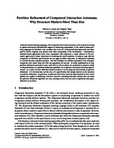
The scaling of the system with respect to data size is very important to measure. We tried to show that given two similar MPI parallel programs, one of which relies on SCIRun2 for data redistribution and the other does not require redistribution of any kind, the overhead imposed by the system’s data redistribution will be more negligible as the problem size gets larger. We compared and plotted the difference factor of the running time of the SCIRun2 componentized application and the simple MPI implementation. Figure 5.1 shows the results of this experiment. Tables 5.1, 5.2, and 5.3 show the experiment times of Jacobi’s, LU Factorization, and Odd-Even Sort algorithm respectively. The LU Factorization is represented by the line furthest to the left. The middle line represents the Jacobi algorithm, whereas the line on the right is the Odd-Even Merge Sort. The graph’s problem size for LU Factorization and Jacobi represent one side of a
38
Table 5.3. Odd-Even Sort running times using four parallel processes. Problem Size MPI Time SCIRun2 Time MPI Time / SCIRun2 Time 500 0.001113 0.010483 9.41868823 1000 0.001173 0.011189 9.538789429 2000 0.002381 0.016644 6.990340193 5000 0.003774 0.032934 8.726550079 10000 0.016741 0.063244 3.777791052 50000 0.043401 0.148052 3.411257805 100000 1.201013 3.003914 2.501150279 Times are in seconds. 30
SCIRun2 runtime / MPI runtime
25
20 Jacobi LU Factor OE Sort
15
10
5
0
1
10
100
1000
10000
100000
Problem Size
Figure 5.1. System scaling graph. square matrix. Odd-Even Merge Sort uses one-dimensional arrays, the size of which is depicted as the problem size in this graph. It is clearly noticeable that as the problem size increases, the factor of the difference between the SCIRun2 and MPI programs decrease. This decrease does not in any way suggest that the overhead imposed by the redistribution remains static as the problem space grows. In fact, we claim that this is the case due to an increase in data to be transferred over the network. Other overheads that SCIRun2 imposes are connected to the underlying system structure. The system is heavily multithreaded in order to always achieve reasonable response time; therefore a substantial performance penalty is paid for
39 thread management. However, the schedule calculation, the PRMI, and other time costs are static, and we see that the overall overhead becomes less and less important as the data increases. To show this, we measured the number of bytes of data sent from the callee to the caller component in the Jacobi example. There were a 103 bytes of overhead data that were sent from the callee component. These include the data used to calculate the schedule and manage the method invocation. This amount remained static as the problem size grew showing the diminishing importance of the overhead with the growth of the problem size. The next section will attempt to further show this by providing a breakdown of the overhead of SCIRun2’s PRMI and automatic data redistribution.
5.3
Overhead Analysis
The analysis of the overhead our system imposes on the execution of an application has the intention of providing us with a clear picture of our system, therefore allowing improvements to minimize the overhead. We used the characteristic applications we designed to run a series of experiments, noting the exact time required to accomplish the PRMI and M-by-N data redistribution from the perspective of one participating process. One experiment had the intention of partitioning and analyzing the data redistribution on one caller process. The benchmarks were made on an application that was solving a 2000 by 2000 matrix using LU Factorization. The results of this experiment are provided in Figure 5.2. The experiment shows that data marshaling is the most expensive task in the redistribution from the caller perspective. The data are marshaled element by element, constantly requiring the underlying communication library to be invoked. Currently, SCIRun2 relies on the Nexus communication library from the Globus Toolkit [6, 5, 7] for this purpose. The data marshaling is a task whose time share grows as the data grow larger and will be considered as a prime candidate in system optimization. Another interesting aspect of this experiment was the relatively brief time (0.23% of total redistribution time) it took for the system to calculate the redistribution schedule. The total time the caller process took to redistribute the data was 4.74 seconds. We measured 2.66 seconds for a representative callee process to receive and assemble the data in the same application. Another experiment was intended to provide us with a comparison of all of the method invocation possibilities of our system. This test would show the overhead imposed by
40
100.00% 90.00% 80.00% 70.00% 60.00% 50.00% 40.00% 30.00% 20.00% 10.00% 0.00% Marshal Data
Send Data
Calculate Schedule
Figure 5.2. M-by-N overhead analysis. the PRMI and data redistribution system in a separate manner. We used the same representative application as above and timed the following invocations: serial invocation, independent PRMI, collective PRMI (without M-by-N), and collective PRMI with 400 byte M-by-N arrays. The resulting data are located in Table 5.4. The data shown by this experiment clearly represent that the M-by-N redistribution is much more costly than the PRMI itself. Similarly, a very small amount of the M-by-N data redistribution cost comes about by the requirements in the PRMI handling. This in turn shows that the performance of the system is highly dependent on optimizing the redistribution feature.
Table 5.4. Invocation comparison. serial invocation independent PRMI collective PRMI (without M-by-N) collective PRMI (with 400 byte M-by-N arrays)
Method Invocation Time 432.6 550 1539 5427
Times are in microseconds.
41
5.4
Comparison to Similar Systems
In this section, we attempt to compare SCIRun2’s performance to that of other existing systems. SCIRun2’s functionality is unique in the way it treats components similarly to established component standards and in the way it uses the IDL to provide automatic data redistribution. A system that provides these functionalities in a closely similar way does not exist. However, we chose to compare SCIRun2’s performance to a system that provides data redistribution, regardless of the manner it chooses to do so. We chose Global Arrays [17, 3] as a system that provides asynchronous, one-way communication which can provide a user with similar functionality to that of M-by-N data redistribution. This toolkit used the concept of a global array to create a environment similar to shared-memory for distributed-memory architectures. Global Arrays are well implemented and are widely used for similar applications to that of SCIRun2.
We
programmed the LU Factorization application using the Global Arrays toolkit to perform a data redistribution pattern similar to that of the SCIRun2 version of this application. Both implementations were based on MPI to perform the actual LU Factorization algorithm. Table 5.5 and Figure 5.3 show the execution time comparison of this experiment. The experiment shows that the Global Arrays implementation has a high starting/initialization overhead. However, as the problem space grows we see that the overhead grows at a much smaller pace than that of SCIRun2, resulting with a faster time for the Global Arrays 600x600 matrix LU Factorization. The Global Arrays toolkit has highly optimized communication primitives that are tailored specifically to separate environments. The communication of SCIRun2 is one specific area that requires improvement in order to match the data transfer performance of the Global Array toolkit.
Table 5.5. Global Arrays comparison of LU Factorization algorithm running times using four parallel processes. Problem Size Global Arrays Time SCIRun2 Time 40x40 1.011828 0.027201 100x100 1.033565 0.123307 160x160 1.093734 0.502175 200x200 1.450243 0.676691 320x320 1.843234 1.308741 600x600 5.701233 6.2124 Times are in seconds.
42
700 600
Problem Size
500 400
Global Arrays SCIRun2
300 200 100 0 0
1
2
3
4
5
6
7
Seconds
Figure 5.3. Arrays.
Comparison of LU Factorization performance of SCIRun2 and Global
CHAPTER 6 CONCLUSIONS AND FUTURE RESEARCH The SCIRun2 system has demonstrated that M-by-N data redistribution based on PRMI with the help of an IDL compiler is a tool that can benefit a scientific component programmer. Further, this system described a method to put all of this functionality in the IDL compiler and its associated runtime objects. In order to accomplish this, we described a paradigm for PRMI. Our goal was to illustrate a way of handling PRMI that would be simple, while encompassing most invocation scenarios. We described our additions to the CCA Scientific IDL (SIDL) that could be used to tailor the method invocation to the appropriate need. We also provided two methods to report a component’s data distribution at runtime. This would enable the distribution to adapt to the number of parallel processes without modification to the code. We described our implementation as well as some of the major algorithms we used to provide all of the functionality we described, such as the index intersection in order to calculate the data redistribution schedule. Finally, we showed performance results concerning different aspects of our system. These included experiments regarding system scaling, overhead analysis and comparison with the Global Arrays system. We showed that the system scales well and that most of the overhead is static. The redistribution of the data took a considerable amount of time and was the only overhead that grew with the size of the problem. Overall, we feel that this was acceptable behavior given the functionality that SCIRun2 tries to provide. The overhead analysis showed that the network traffic was, again, mostly data redistribution. Other networking overheads were small and static. The approach to data marshaling and the underlying communication infrastructure are a slowing point. This is one aspect that we plan to focus on in the future. The Global Arrays system was slower than SCIRun2 for very small problems, but was increasingly faster as the problem space grew. We believe that this is due to the Global Arrays architecture-specifically optimized
44 communication library. SCIRun2 needs a significant deal of improvement in that area in order to increase its overall performance. The future work of this project also involves permeating our PRMI and M-by-N redistribution infrastructure through the component framework and GUI (Graphical User Interface) of SCIRun2. In addition, we plan on adding less constrained distribution descriptions. These would allow a user to partially specify a distribution and the system will adapt according to the available specifications. This would allow deployed components to be more flexible to the amount of data they are distributed. Finally, we plan on devising and implementing methods that would further improve the performance of our system.
APPENDIX A SIDL INTERFACES TO EXAMPLE APPLICATIONS In the following we show the SIDL interfaces describing the example applications we discussed. These interfaces are compiled through the SCIRun2 SIDL compiler to provide the functionality I have discussed in this thesis.
A.1
Jacobi Solution to the Laplace Heat Equation
package Jacobi_ns { distribution array X ; interface Jacobi { int solveHeatEquation(inout X arr,in double top,in double bottom, in double left,in double right); }; };
A.2
LU Matrix Factorization
package LUFactor_ns { distribution array A ; interface LUFactor { int LUFactorize(in A arr); }; };
A.3
Odd-Even Merge Sort
package OESort_ns { distribution array X ; distribution array Y ;
46 distribution array Z ;
distribution array A ;
interface OESort { int sort(in X arr, out Y odds, out Z evens); }; interface OESplit { int split(inout A arr); }; };
APPENDIX B SOURCE CODE TO ODD-EVEN MERGE SORT The Odd-Even Merge Sort algorithm relies heavily on data transfers. Its implementation can rely on our system to perform these distributions, therefore aleviating this responsibility from the programmer. Below, we will show how this algorithm would be implemented using our system to perform the data transfer. The implementation is not recursive and limited to sorting two lists. We will also show an MPI implementation of this algorithm in order to compare that the SCIRun2 implementation is simpler to program. The other benchmarks illustrated have similar differences, namely that the MPI implementations are more complex and less flexible in regard to data distribuions than those expressed using our system.
B.1
SCIRun2 Implementation B.1.1
OESplit Caller
//Generate a random number list init(arr,ARRSIZE);
//Inform everyone else of my distribution //(this sends a message to all the callee objects) Index** dr0 = new Index* [1]; dr0[0] = new Index(0,ARRSIZE,1); MxNArrayRep* arrr0 = new MxNArrayRep(1,dr0); oesplit_proxy->setCallerDistribution("A",arrr0);
/*Odd-Even merge sort start*/ oesplit_proxy->split(arr);
48
B.1.2
OESplit Callee
OESplit* oesplit=new OESplit;
int localsize = ARRSIZE / mpi_size; int sta = mpi_rank * localsize; int fin = sta + localsize; if (mpi_rank == mpi_size-1) fin = ARRSIZE;
//Set up server’s requirement of the distribution array Index** dr10 = new Index* [1]; dr10[0] = new Index(sta,fin,1); MxNArrayRep* arrr10 = new MxNArrayRep(1,dr10); oesplit->setCalleeDistribution("A",arrr10);
int OESplit::split(const array& arr) { /*Pairwise check of merged array:*/ for(unsigned int arri = 0; arri+1 < arr.size(); arri+=2) if (arr[arri] > arr[arri+1]) { int t = arr[arri]; arr[arri] = arr[arri+1]; arr[arri+1] = t; } }
B.1.3
OESort Caller
Index** dr0 = new Index* [1]; dr0[0] = new Index(sta,fin,1); MxNArrayRep* arrr0 = new MxNArrayRep(1,dr0); oesort_proxy->setCallerDistribution("X",arrr0);
Index** dr1 = new Index* [1]; dr1[0] = new Index(sta,fin,2);
49 MxNArrayRep* arrr1 = new MxNArrayRep(1,dr1); oesort_proxy->setCallerDistribution("Y",arrr1);
Index** dr2 = new Index* [1]; sta = abs(mpi_rank-1) * localsize; fin = sta + localsize; dr2[0] = new Index(sta+1,fin,2); MxNArrayRep* arrr2 = new MxNArrayRep(1,dr2); oesort_proxy->setCallerDistribution("Z",arrr2);
oesort_proxy->sort(arr,odds,evens);
B.1.4
OESort Callee
OESort* oesort=new OESort;
int localsize = ARRSIZE / mpi_size; int sta = mpi_rank * localsize; int fin = (mpi_rank * localsize) + localsize; if (mpi_rank == mpi_size-1) fin = ARRSIZE;
//Set up server’s requirement of the distribution array Index** dr0 = new Index* [1]; dr0[0] = new Index(sta,fin,1); MxNArrayRep* arrr0 = new MxNArrayRep(1,dr0); oesort->setCalleeDistribution("X",arrr0);
Index** dr1 = new Index* [1]; dr1[0] = new Index(sta,fin,1); MxNArrayRep* arrr1 = new MxNArrayRep(1,dr1); oesort->setCalleeDistribution("Y",arrr1);
Index** dr2 = new Index* [1]; dr2[0] = new Index(sta,fin,1);
50 MxNArrayRep* arrr2 = new MxNArrayRep(1,dr2); oesort->setCalleeDistribution("Z",arrr2);
int OESort::sort(const array& arr, array& odds, array& evens) { mergeSort(arr,evens,odds); return 0; }
B.1.5
MPI Implementation
int my_rank, nodes, i_size; int* destarr; int* merge_arr; int* arr;
MPI_Init(&argc,&argv);
MPI_Comm_rank(MPI_COMM_WORLD,&my_rank); MPI_Comm_size(MPI_COMM_WORLD,&nodes);
/*Allocate Array:*/ i_size = ARR_SIZE/nodes; arr = (int*)malloc(i_size*sizeof(int));
/*Each process generates a random number list and sorts it*/ generate(arr,i_size); sort(arr, arr+i_size);
for(int k=1; k < nodes ;k=k*2) { if ((my_rank == 0) || ((my_rank % (k*2)) == 0)) { if (my_rank+k < nodes) { /*Receive size of array:*/ int destsize;
51 MPI_Recv(&destsize, 1, MPI_INT, my_rank+k, 0, ...);
/*Receive array:*/ destarr = (int*)malloc(destsize*sizeof(int)); MPI_Recv(destarr, destsize, MPI_INT, my_rank+k, 1, ...);
/*Merge:*/ int m_size = i_size + destsize; merge_arr = (int*)malloc(m_size*sizeof(int)); int loc,i,j;
/*Odd-Even -> Even*/ loc=0; i=0; j=1;
while (i < i_size) { if (j < destsize) { if (arr[i] < destarr[j]) { merge_arr[loc] = arr[i]; i+=2; } else { merge_arr[loc] = destarr[j]; j+=2; } } else { merge_arr[loc] = arr[i]; i+=2; } loc+=2; }
52 while (j < destsize) { merge_arr[loc] = destarr[j]; loc+=2; j+=2; }
/*Even-Odd -> Odd*/ loc=1; i=1; j=0; while (i < i_size) { if (j < destsize) { if (arr[i] < destarr[j]) { merge_arr[loc] = arr[i]; i+=2; } else { merge_arr[loc] = destarr[j]; j+=2; } } else { merge_arr[loc] = arr[i]; i+=2; } loc+=2; } while (j < destsize) { merge_arr[loc] = destarr[j]; loc+=2; j+=2; }
53 /*Pairwise check of merged array:*/ for(loc = 0; loc+1 < m_size; loc+=2) if (merge_arr[loc] > merge_arr[loc+1]) { int t = merge_arr[loc]; merge_arr[loc] = merge_arr[loc+1]; merge_arr[loc+1] = t; }
else if ((my_rank % k) == 0) { /*Send size of array:*/ MPI_Send(&i_size, 1, MPI_INT, (my_rank-k), 0, MPI_COMM_WORLD); /*Send array:*/ MPI_Send(arr, i_size, MPI_INT, (my_rank-k), 1, MPI_COMM_WORLD); } }
MPI_Finalize();
REFERENCES [1] Armstrong, R., Gannon, D., Geist, A., Keahey, K., Kohn, S., McInnes, L., Parker, S., and Smolinski, B. Toward a common componnent architecture for high-performance scientific computing. In Proceedings of the 8th IEEE International Symposium on High Performance Distributed Computation (July 1999). [2] Beckman, P. H., Fasel, P. K., Humphrey, W. F., and Mniszewski, S. M. Efficient coupling of parallel applications using PAWS. In Proceedings of the 7th IEEE International Symposium on High Performance Distributed Computation (July 1998). [3] Chen, Y., Nieplocha, J., Foster, I., and Winslett, M. Optimizing collective i/o performance on parallel computers: a multisystem study. In Proceedings of the 11th international conference on Supercomputing (1997), pp. 28–35. [4] Epperly, T., Kohn, S., and Kumfert, G. Component technology for highperformance scientific simulation software. In Working Conference on Software Architectures for Scientific Computing Applications (Ottawa, Ontario, Canada, October 2000), International Federation for Information Processing. [5] Foster, I., Karonis, N., Kesselman, C., Koenig, G., and Tuecke, S. A secure communications infrastructure for high-performance distributed computing. In Proceedings of the 6th IEEE International Symposium on High Performance Distributed Computation (July 1997). [6] Foster, I., and Kesselman, C. Globus: A metacomputing infrastructure toolkit. The International Journal of Supercomputer Applications and High Performance Computing 11, 2 (Summer 1997), 115–128. [7] Foster, I., Kesselman, C., and Tuecke, S. The Nexus approach to integrating multithreading and communication. Journal of Parallel and Distributed Computing 37, 1 (1996), 70–82. [8] Geist, G. A., Kohl, J. A., and Papadopoulos, P. M. CUMULVS: Providing fault-tolerance, visualization and steering of parallel applications. In Environment and Tools for Parallel Scientific Computing Workshop (Domaine de Faverges-de-laTour, Lyon, France, August 1996). [9] Group, O. M., 2002. [10] Johnson, C. R., and Parker, S. G. The scirun parallel scientific computing problem solving environment. In Ninth SIAM Conference on Parallel Processing for Scientific Computing (1999).
55 [11] Johnson, C. R., Parker, S. G., and Weinstein, D. Large-scale computational science applications using the scirun problem solving environment. In Supercomputer 2000 (2000). [12] Keahey, K., Fasel, P. K., and Mniszewski, S. M. PAWS: Collective invocations and data transfers. In Proceedings of the 10th IEEE International Symposium on High Performance Distributed Computation (July 2001). [13] Kohn, S., Kumfert, G., Painter, J., and Ribbens, C. Divorcing language dependencies from a scientific software library. In Proceedings of the 10th SIAM Conference on Parallel Processing (Portsmouth, VA, March 2001). [14] Leighton, F. T. Introduction to Parallel Algorithms and Architectures. Morgan Kaufmann Publishers, Inc., 1992. [15] Maassen, J., Kielmann, T., and Bal, H. E. GMI: Flexible and efficient group method invocation for parallel programming. Tech. rep., Faculty of Sciences, Division of Mathematics and Computer Science, Vrije Universiteit, Amsterdam, The Netherlands, 2001. [16] Musser, D. R., Derge, G. J., and Saini, A. STL Tutorial and Reference Guide: C++ Programming with the Standard Template Library. Addison-Wesley Publishing Company, 2001. [17] Nieplocha, J., Harrison, R. J., and Littlefield, R. J. Global Arrays: a portable ‘shared-memory’ programming model for distributed memory computers. In Proceedings of Supercomputing ’94 (November 1994), pp. 340–349. [18] Parker, S. G. The SCIRun Problem Solving Environment and Computational Steering Software System. PhD thesis, The University of Utah, August 1999. [19] Parker, S. G., Beazley, D., and Johnson, C. R. Computational steering software systems and strategies. IEEE Computational Science and Engineering 4, 4 (1997), 50–59. [20] Parker, S. G., and Johnson, C. R. Scirun: A scientific programming environment for computational steering. In Proceedings of Supercomputing ’95 (December 1995). [21] Rosen, K. H. Elementary Number Theory and Its Applications. Addison-Wesley Publishing Company, 1984. [22] Szyperski, C. Component Software: Beyond Object-Oriented Programming. Addison-Wesley Publishing Company, 1998.