Parallel Computer Architectures and Problem Solving Strategies for ...

IEEE TRANSACTIONS ON COMPUTERS, VOL. c-34, NO. 11, NOVEMBER 1985

973

Parallel Computer Architectures and Problem So1ving Strategies for the Consistent Labeling Pr JEANETTE TYLER McCALL, JOSEPH G. TRONT, SENIOR MEMBER, IEEE, F. GAIL GRAY, 4IOR MEMBER, IEEE, NOV 1 4 1985 ROBERT M. HARALICK, FELLOW, IEEE, AND WILLIAM M. McCORMACI Parallel computer architectures and problem solving strategies for the consistent labeling problem are studied. Problem solving factors include: processor intercommunication methods, passing order, and selection of the initial processor to receive the problem. A Pascal program is used to simulate multiprocessor systems. The simulation is set up so that the parameters affecting the problem solving factors can be varied. The simulations were restricted to eight-processor systems. Simulation results were analyzed using the statistical analysis package called SAS. The results show that interprocessor communications are best performed using an interrupt system, as opposed to a polling system. Transfers of work should be directed randomly. It is best to choose an initial processor with a small maximum distance of any processor in the architecture from the initial processor. Large diameter architectures and architectures with very few buses perform poorly. Index Terms -Computer simulation, consistant labeling problem, parallel architectures, problem solving strategies, processor Abstract

MURRAY HILL UBRARY

polynomial solution is found for any _T olIAg RI l I , then all NP-complete problems will be able to be solved in polynomial time. Other NP-complete problems are the traveling salesman problem [1], the scene labeling problem [4], the graphy clique problem [1], the graph homomorphism problem [5], and propositional logic problems. Although most of the work done on solving the consistent labeling problem has been for single processor systems [8], the consistent labeling problem is well suited to parallel solution because it is easily divided into mutually exclusive subproblems. To represent our architectures, we have chosen the bipartite graph. A graph is bipartite if its nodes can be partitioned into two disjoint subsets such that every link in the graph connects a node in one subset with a node in the other subset. We let the processors be one subset of nodes and buses be the other subset. A link between a processor node intercommunication. and a bus node means that the processor arid bus are conI. INTRODUCTION nected. The degree of a node is the number of links attached I N this paper we will be examining parallel computer archi- to that node. Therefore, a processor's degree is the number of tectures and problem solving strategies for the con- buses attached to that processor and a bus' degree is the sistent labeling problem. We will not be studying how the number of processors attached to the bus. In our work, we have restricted ourselves to regular archiproblem gets loaded into the architecture or how the solutions tectures because they are more easily implemented in VLSI. are sent back out as these are more networking problems. In architectures each of the processors has the same regular First of all, let us define the consistent labeling problem. each of the buses has the same degree. This would and degree Let us assume we have N units (variables) and M labels mask to be built using an overlay strucallow production the (values). Let U be the set of units and L be the set of labels. we are not considering general restriction this using ture. By Let R be a unit-label constraint relation. R can be repwe are not considering a few also, connection and networks, resented as a binary relation on U x L:R E (U X L)2. The the buses and processors which in of networks regular types consistent labeling problem [4], [8] is to find all functions have the same degree as not on of do the the network fringe f:U -- L satisfying that for all (u,v) G U x U, (u,f(u), restricted ourselves further have We in [ middle 101. those the v,f(v)) E R. Less formally, the consistent labeling problem number of archithe make to to architectures eight-processor involves searching and matching. The object is to give all of the units (objects) unique labels that satisfy. certain require- tectures to be examined manageable. Future studies will examine architectures with a larger number of processors. We ments that are specified by the relation R. that many of the results obtained by studying eightexpect One important characteristic of the consistent labeling architectures will be valid for larger architectures. processor problem is that it is an NP-complete problem. NP-complete the general operation of a parallel comconsider Let us problems typically take exponential time to solve, but if a puter. One processor initially receives a large problem to Manuscript received June 1, 1984; revised April 22, 1985. solve. This initial processor divides the problem up and gives J. T. McCall was with the Department of Electrical Engineering, Virginia Polytechnic Institute and State University, Blacksburg, VA. She is now with subproblems to its neighboring processors. From there on, processors with extra work give subproblems away to their the IBM Corporation, Mannassas, VA 22110. J. G. Tront and F. G. Gray are with the Department of Electrical Engineer- idle neighbors. Processors with no idle neighbors begin solving, Virginia Polytechnic Institute and State University, Blacksburg, VA ing their problem. When all of the processors have work, they 24061. continue UniverState working until a processor becomes idle. A neighand Institute was Polytechnic R. M. Haralick with the Virginia sity, Blacksburg, VA. He is now with Machine Vision International, Ann boring processor with extra work will give work to an idle Arbor, MI 48104. W. M. McCormack is with the Department of Electrical Engineering, Vir- processor. By the term extra work we mean that the processor has a subdividable problem (work that it could give away). ginia Polytechnic Institute and State University, Blacksburg, VA 24061. 0018-9340/85/1100-0973$01.00 © 1985 IEEE

974

IEEE TRANSACTIONS ON COMPUTERS, VOL.

Requirements for such a system are the following. 1) Processors must be capable of subdividing their problem. 2) Processors with extra work must be capable of transferring subproblems to their idle neighbors. 3) The basic algorithm in each processor must be the same and must be such that each processor could solve the entire problem alone. Note that the algorithm is the same, but the processors are running asynchronously. We used a multiprocessor simulation program [7] which met these requirements to examine the effects of various problem-solving factors and architectural factors on system performance. The information generated by the simulator was analyzed with the Statistical Analysis System (SAS) package. Further information on the material covered in this paper can be obtained in the thesis of [10]. II. PROBLEM SOLVING FACTORS

In a parallel system certain problem-solving factors need to be considered. Some of these factors include how the problems should be subdivided, how the need to transfer work should be recognized, and the algorithm that should be used to solve the problem. From previous results [6], [7] we know that a forward checking algorithm is better than backtracking. It is also better to have processors with extra work transfer large problems rather than small ones to their idle neighbors. A depthfirst search is better than a breadth-first search because it leaves larger problems available for transfer. The previous simulation results also showed that it is best for processors with extra work to transfer half of their problem to their idle neighbor. The following sections provide definitions and explanations for the various problem-solving factors. A. Processor Intercommunication Processor intercommunication is the first problem-solving factor examined in this paper. Processor intercommunication deals with how the need to transfer work is recognized. We considered two interrupt systems and one polling system. The first interrupt system we considered was called the Bus Method. In the Bus Method, it is the bus that is responsible for arranging a transfer of work between a processor with extra work and an idle processor. In the second interrupt technique, called the Idle Processor Method, it is the idle processor that is responsible for arranging a transfer of work by finding a bus that is not busy and a processor with extra work. In the Polling Method, processors with extra work regularly poll their neighbors to see if any of them are idle. The Bus Method would require a "smart bus," whereas the other two methods could use a "dumb bus" such as a shared memory. An additional parameter needed to fairly compare the different types of processor intercommunication is the time it takes a device (processor or bus) to check around and determine whether or not a transfer of work needs to take place. This parameter will be called time to check and will be de-

c-34, NO. 1I, NOVEMBER 1985

noted as Tchk. Tchk will provide the simulator with a relative rather than an absolute measure of time. B. Passing Order Passing order deals with how the transfer of work is directed. Work should be passed from the outskirts of the architecture towards the center, or from the center to the outskirts, or should all choices of transfer direction be made randomly. We call the passing order described Central, Noncentral, and Random, respectively. (By Noncentral we do not imply the term distributed, but rather we mean "other than the geometric center.") To see how the different passing orders work with the different types of processor intercommunicatiolz methods refer to the following examples. Example I -Polling Method: Let the processors and buses in Fig. 1 be a part of an architecture. Suppose processor A has extra work and processors E, B, and C are idle. Also suppose that BUS 1 is closer to the center of the architecture than BUS2 and that processor C is closer to the center of the architecture than processor B. If the passing order were Central, processor A would choose BUSI, and BUS1 would choose processor C. Example 2 -Idle Processor Method: Let processor A be idle and processors E, B, and C have extra work. Again, suppose BUS 1 is closer to the center of the architecture and that the passing order is Central. Since the passing order is Central, we want the work to be passed from the outskirts towards the center. Since BUS2 is less central than BUS1, BUS2 is chosen, and therefore processor E is chosen. Example 3 -Bus Method: Suppose processor A is idle and processors B, C, and E have extra work. Let the passing order be Random. A is the only idle processor, so both BUS 1 and BUS2 want A. Suppose BUS I recognizes that processor A is idle before BUS2 makes this same recognition. BUSI gets processor A and randomly chooses between processors B and C to determine which of them will send work to processor A.

C. Starting Point The starting point is the processor which initially begins work on the problem. In an attempt to determine which processor provides the best starting point, we divided the set of processors.into distance vector classes (defined below). For each architecture, we selected one processor from each distance class, and these became the tested starting points for that architecture. The tested starting points are hereafter referred to as the starting points. The problem is instantiated in the starting point processor and is then passed from processor to processor according to the problem passing strategy. The following definitions are useful. 1) Diameter: Length of the longest path in the graph. 2) Distance Vector (Signature): An n-dimensional vector, where n is the diameter of the graph, that describes a node's proximity to other nodes in the graph. A node with distance vector (dv 1, dv2, dv3,... , dvn) has dvl nodes it reaches by a path of length 1, dv2 nodes which it can reach

MC CALL et

al.:

975

PARALLEL COMPUTER ARCHITECTURES

/

architecture might be helpful in getting the problem to spread out evenly among the processors initially. This would hopefully keep the processors busy longer, before they started running out of work.

/

IV. SIMULATION EXPERIMENTS /

Fig. 1. Portion of processor interconnection scheme.

by a path of length 2 but not by a path of length 1, dv3 nodes which it can reach by a path of length 3 but not by a shorter path, and so on. 3) Distance Vector Class: A group of processors, within an architecture, that all have the same distance vector. III.

ARCHITECTURAL FACTORS

Architectural factors are characteristics of an architecture that can be parameterized (given numerical values). We examined various factors to evaluate their usefulness in predicting architecture performance. The architectural factors we examined are listed and defined below. 1) Architecture Class: A group of architectures which all have the same number of processors, processor degree, number of buses, and bus degree. The notation AC(np, dp, nb, db) denotes an architecture class with np processors, nb buses, a processor degree of dp, and a bus degree of db. 2) Other Architectural Factors Examined: a) Diameter -(defined previously); b) Average Distance -the average distance between nodes in the graph; c) Average Distance Vector (Signature) -an ndimensional vector, where n is the diameter of the graph, that is an average of the distance vectors of all the nodes in the graph; d) Number of automorphism classes -the number of nodes in the graph (architecture) which are structurally distinct from each other. Diameter, average distance, and average distance vector are all measures of the nodes' (processors or buses) proximity to other nodes in the graph (architecture). The number of automorphism classes is a measure of the symmetry of the graph. The fewer the number of automorphism classes the more symmetric the graph is. Having the nodes in the graph close to each other would help to spread the problem throughout all the nodes quickly. It would also make it more likely for idle processors to be able to get work from a processor with extra work when the problem is dying out and there are not many processors with extra work available. A symmetric

A. Problem-Solving Factors For all of the experiments the analysis of variances and the regression analyses were done using the General Linear Model (GLM) procedure of the SAS package. In all cases the null hypothesis is tested and the PR > F is the probability that the source does not affect performance. In all cases, including the Duncan's ranking, we are requiring a PR > F of 0.05 or lower before we are considering a source significant. 1) Processor Intercommunication: a) Experiment goals: The goals of this experiment are 1) to determine which processor intercommunication method is best, and 2) to determine how sensitive polling and interrupt systems are to varying values of the Tchk parameter. Due to the number of unsettled problem solving factors, the number of architectures involved in this experiment was reduced to a minimum. Although the architectures we have selected give some variety, there are too few architectures to make any conclusions about the effect of parameters that have a significant interaction with architecture type. Therefore, if any valid conclusions are to be made in this experiment, the results must show no interaction between processor intercommunication method and architecture type, and no interaction between Tchk and architecture type. b) Experiment design: In this experiment, processor intercommunication vwas tested at three levels, corresponding to the three methods discussed in Section Il-A. Tchk was tested at two levels (one increment of time and five increments of time -small and large). Based on the previous experiments [3], we have determined that it is best to use a forward checking algorithm, use a depth-first search, and have processors pass 50 percent of their work. All experiments used these parameters. In order for the results to be applicable for different problem sizes and architectures, and different starting points within the architectures, two problem sizes (small and large) and eleven different architectures were used. Each architecture was run with each of its starting points. The architectures were selected from the architecture classes AC(8, 3, 12, 2), AC(8, 3, 6, 4), AC(8, 3, 4, 6), AC(8, 2, 8, 2), and AC(8, 7, 28, 2). Finally, one replication was run for each combination. This involves running the simulation with different random number seeds to create statistically equivalent combinatorial problems. An analysis of variance was used to determine the significance of the problem-related parameters and to determine interactions of parameters. The measure of performance was speedup (over a single processor system). c) Results: The SAS analysis showed that the processor intercommunication method and Tchk are significant at the 0.0001 level. By examining Table I, we see that Polling is worse than the interrupt systems for each passing order. We

976

IEEE TRANSACTIONS ON COMPUTERS, VOL. c-34, NO. 11, NOVEMBER 1985

TABLE I Duncan's Grouping by Passing Order, Nunit, and Tchk

I

Noncentral

Random

Central

112 112 120 120 112 112 120 120 112 112 120 120 lI s 1 s 1_5 1 1 s 1 5

Nuni t

I1

Tchk Bus

IdlePr

I_A

A_

A_ IA

A

A

A

I

Polling

A

AIAIAIA

I_A

1

A

A

A

A

A

|A

A

B

B

A

II __

__

A

A

A

B

AIAIlIAIAIAIAIA I_I

A B

I_

__

Examining the Interaction Between Processor Intercom. & Tchk Mean

Tchk

A

7.4169

5

BUS

A

7.4096

1

BUS

A

7.4011

5

IDLEPR

A

7.3887

1

IDLEPR

Duncan Grouping

B

7. 3618

B

C

7.2185

Processor Intercom.

POLLING

5

POLLING

can also see that the Bus Method is significantly better than the Idle Processor Method for all passing orders except Random. This means that if Random proves to be the best passing order, either of the two interrupt systems are acceptable, but if either Noncentral or Central is the best passing order, then the Bus Method is the best processor intercommunication method. Table I shows that varying the value of Tchk does not make a significant difference for the interrupt systems. In interrupt systems, the only effect a longer time to check has on performance is that it is slightly longer before the idle processors receive work. But, in polling systems, the processors with extra work are having to regularly take time away from working to check for idle neighbors. This regular checking is what makes polling systems sensitive to the value of Tchk. 2) Passing Order: a) Experiment design and goals: The goal of this experiment was to determine the best passing order. Passing order was tested at three levels: Central, Noncentral, and Random. Based on the previous experiments discussed by Gray et al. [3] in Section IV-A1) we have determined that it is best to use a forward checking algorithm, use a depth-first search, and have processors pass 50 percent of their work. We have also determined that the best overall processor intercommunication method is the Bus Method. All experiments used these parameters. In order for the results to be applicable for different problem sizes, different architectures, and different starting points within the architectures, 2 problem sizes (small and large) and 69 different architectures were used. Each architecture was run with each of its possible starting points. The architectures were from the architecture classes AC(8, 3, 12, 2), AC(8, 3, 6, 4), and AC(8, 5, 10, 4). The different architec-

ture classes were chosen to achieve a variety of processor degrees and bus structures. For the architecture classes AC(8, 3, 12, 2) and AC(8, 3, 6, 4), all nonisomorphic architectures were selected. This resulted in 19 architectures for the architecture class AC(8, 3, 12, 2) and 27 architectures for the AC(8, 3, 6, 4). For the architecture class AC(8, 5, 10, 4), only the more symmetric nonisomorphic architectures were chosen, due to the large number of architectures. The more symmetric architectures were selected by choosing architectures with 19 or fewer automorphism classes of nodes (including processors and buses) since this resulted in a reasonable number (23) of nonisomorphic architectures. Finally, one replication was run for each combination. This involves running the simulation with different random number seeds to create statistically equivalent problems. An analysis of variance was used to determine the significance of the problem related parameters. The measure of performance was speedup (over a single processor system). One complication arose when we first tried to run the experiment. The memory requirement was larger than the user is allowed. This problem was caused by the large number of architectures and the way SAS solves analysis of variance problems. Instead of an overall analysis, we divided the data by architecture class and analyzed the result for each architecture class separately. b) Results: Passing order made a significant difference for both the architecture class AC(8, 3, 6, 4) and the architecture class AC(8, 5, 10, 4). The buses in the architecture class AC(8, 3, 12, 2) have only two processors attached to them. When they have one processor that is idle and one processor with extra work they have no choice in transfer direction. Therefore, the result that passing order is not significant for the architecture class AC(8, 3, 12, 2) makes sense. For both architecture classes AC(8, 3, 6, 4) and AC(8, 5, 10,4), the passing order Random was significantly better than the other two passing orders. Refer to Table II. Since Random is the best passing order, the two interrupt systems do not perform significantly different from each other. 3) Starting Point: This experiment was the last to be completed. As such, it refers to some of the results of Section IV-B (Architectural Factors). You may wish to wait to read this section until after reading the Architectural Factors results, but it is not necessary for an understanding of the material covered in this section. a) Experiment Goals and Design: The goal of this experiment is to optimally select which processor, within an architecture, initially begins work on the problem. For each architecture, we have divided the processors into Distance Vector Classes. Processors which have the same distance vector are said to be in the same distance vector class. For any given architecture, we have decided to select one processor from each distance vector class and have those processors be the starting points, i.e., the processors at which we will try starting the problem. The parameters that we will be using are the distance vector of a processor and a parameter which we will call MaxDis (the maximum distance of any node from the processor). Based on previous experiments discussed by Gray et al. [3] and in Sections IV-A1) and 2), we have determined that

977

MC CALL et al.: PARALLEL COMPUTER ARCHITECTURES

Duncan

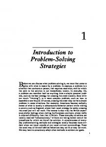
TABLE II

TABLE III

Duncan Grouping for AC(8,3,6,4)

AC(8,3,12,2) Comparison of Architectural Factors

Grouping

Mean

Passing Order

R-Square Value of Problem Size A

7. 6330

Random

B

7.6112

Central

B

7. 6077

Noncentral

Duncan Grouping for AC(8,5,10,4) Duncan

Grouping

Mean

R-Square Value

Amount Above PS-A R-Square

Percentage Predicted

Dist. Vec.

0.932732

0.092433

100.0000

MaxDis

0.902204

0.061905

Random

B

7.6392

Noncentral

B

7. 6369

Central

66.9728

l_

AC(8,3,16,4) Comparison of Architectural Factors

R-Square Value of Problem Size 7.6625

Architecture : 0.840299

Starting Pt. Factor

Passing Order

A

-

-

Architecture : 0.948035

Amount Above I Percentage Predicted PS-A R-Square

Starting Pt. Factor

R-Square Value

Dist. Vec.

0.964489

0.016454

100.0000

MaxDis

0.960335

0.012300

74.7539

._

l__

l__

it is best to use a forward checking algorithm, to use a depthfirst search, to have processors pass 50 percent of their work, and to randomly make all choices on how to direct transfers do not expect MaxDis to be able to predict all that distance of work. The Bus Method of processor intercommunication vector can predict. To determine the percentage of the variavector that was chosen so that we could use data generated for the tion between observations predicted by distance R-Square the examined MaxDis we can be by predicted passing order experiment. All experiments used these is a measure value The R-Square models. two values of the parameters. In order for the results to be applicable to different archi- of the amount of the variation between observations that can tectures and problem sizes, 2 problem sizes (small and large) be accounted for by the model. We did not directly compare and 76 different architectures were used. The architectures the two models' R-Square values because in both of the of the were selected from the architecture classes AC(8, 3, 12, 2), models problem size and architecture account for most associated R-Square the we subtracted Instead, variation. AC(8, 3, 6, 4), and AC(8, 4, 16, 2). The different architecture classes were chosen to achieve a variety of processor with problem size and architecture from the R-Square value degrees and bus structures. For the architecture classes of the two models and compared the resulting values. The results for the architecture classes AC(8, 3, 12, 2) and AC(8, 3, 12, 2) and AC(8, 3, 6, 4), all nonisomorphic archiAC(8, 4, 16, 2) are shown in Table III. For the architecture tectures were selected. This resulted in 19 architectures for class AC(8, 3, 16, 2), MaxDis accounted for 67 percent of the the architecture class AC(8, 3, 12, 2) and 27 architectures for for by distance vector. In the architecture variation accounted the AC(8, 3, 6, 4). For the architecture class AC(8, 4, 16, 2), MaxDis accounted for 74 percent. Although 16, 2), AC(8, 4, only the more symmetric nonisomorphic architectures were does not account for as much variation as distance MaxDis chosen, due to the large number of architectures. The more the MaxDis and performance is between relationship vector, symmetric architectures were selected by choosing architeceach examined, choosing more seen. For architecture easily tures with 8 or fewer automorphism classes of nodes (includMaxDis resulted in a starting a with a small always processor ing processors and buses) since this resulted in a reasonable in For this reason, category. the best performance processor number (30) of nonisomorphic architectures. in selecting startused to be the parameter we chose MaxDis Finally, one replication was run for each combination. ing points. This involves running the simulation with different random number seeds to create statistically equivalent problems. An B. Architectural Factors analysis of variance was used to determine the significance of 1) Factors Within an Architecture Class: the problem-related parameters. The measure of performance a) Experiment goals and design: The goal of this exwas speedup (over a single processor system). Disperiment is to determine which architectural parameters can b) Results: The SAS analysis showed that both tance Vector and MaxDis are significant for the architecture be used to predict performance within an architecture class. classes AC(8, 3, 12, 2) and AC(8, 4, 16, 2). Neither starting The architectural factors examined are diameter, average point (in the previous experiment), distance vector, or Max- distance, the number of automorphism classes, and average Dis was significant for the architecture class AC(8, 3, 6, 4). distance vector. Based on previous experiments discussed by Gray et al. Since the parameter MaxDis can be determined directly and in Sections IV-Al) and 2), we have determined that contains it [3], from the parameter distance vector, and since only to use a forward checking algorithm, to use a depthit is best we in Distance Vector, a subset of the information contained

978

first search, to have processors pass 50 percent of their work, and to have all choices on how to direct transfers of work be made randomly. The Bus Method of processor intercommunication was used so that we could use experiments (simulation runs) that were generated for the passing order experiment. So all experiments used these parameters. In order for the results to be applicable for different architectures and problem sizes, 2 problem sizes (small and large) and 69 different architectures were used. The architectures were selected from the architecture classes AC(8,3, 12, 2), AC(8, 3, 6, 4), and AC(8, 4, 16, 2). Since the same architectures were used for both this experiment and the starting point experiment, we ask the reader to refer to Section IVA3)-a) for further details on the architecture selection. Results from the starting point experiment were not completed by the time of this experiment, so the best starting point, determined by simulation runs, for each architecture was used. Finally, one replication was run for each combination. This involves running the simulation with different random number seeds to create statistically equivalent problems. An analysis of variance was used to determine the significance of the problem-related parameters. The measure of performance was speedup (over a single processor system). We decided that instead of immediately using the SAS package for testing each of the architectural factors, we would rank the architectures and list beside the architectures their corresponding diameter, average distance, etc. This was done to see if there were some factors that could be eliminated, as possible predictors of performance, by inspection. b) Results: The only architectural factor eliminated by using the architecture rankings was the number of automorphism classes, which clearly had no value in predicting performance. The SAS analysis was run for the rest of the architectural factors. The results showed that architecture and all of the architectural factors examined were significant for the architecture classes AC(8, 3, 12, 2) and AC(8, 4, 16, 2). All were not statistically significant for architecture class AC(8, 3,6,4). Since the architectural factors can be determined directly from the architectures, and since they only contain a subset of the information that knowing the architecture itself would provide, we do not expect the architectural factors to predict all that Architecture can predict. The advantage in using the parameters is that they are numeric values, and if we can find a relationship between their values and performance, we will no longer need to examine all architectures in an architecture class. To determine the percentage of the variation between observations predicted by architecture that can be predicted by the architectural factors, we examined the R-Square values of the models. The R-Square value is a measure of the amount of variation between models that is accounted for by the model. We did not directly compare the architecture and the architectural factors models' R-Square values because in both of the models problem size accounts for most of the variation. Instead, we subtracted the R-Square associated with problem size from both of the architecture and architec-

II,

IEEE TRANSACTIONS ON COMPUTERS, VOL. c-34, NO.

NOVEMBER 1985

TABLE IV AC(8,3,12,2) Comparison of Architectural Factors

R-Square Value of Problem Size Alone : 0.906124 Architectural Factor

R-Square

Architecture

Amount Above

Percentage Predicted

0.944403

0.038279

100.0000

Diameter

0.927315

0.021190

55.3567

Average Dist.

0.923818

0.017694

46.2238

DA

0.925324

0.019200

50.1581

Avg.Dist.Vec.

0. 937541

0.031417

82.0737

Value

iNunit R-Square

AC(8,4,16,2) Comparison of Architectural Factors

R-Square Value of Problem Size Alone Architectural Factor

Diameter

0.948128 I

0.937338

0.929642

Amount Above Nunit R-Square

R-Square Value

Architecture

:

0.018486 I

0.007696

Percentage Predicted I

lI

100.0000 41.6315

Average Dist. I

0.936802

0.007160

38.7320

DA

0.937537

0.007895

42.7080

Avg.Dist.Vec.

0.939208 I l__

0.009566 l__

51.7473

l__

tural factors models' R-Squares and compared the resulting values. The results for the architecture classes AC(8, 3, 12, 2) and AC(8, 4, 16, 2) are shown in Table IV. For the architecture class AC(8, 3, 12, 2), average distance vector accounted for the 82 percent of the variation accounted for by architecture. Diameter predicted 55 percent of what ,architecture predicted. For the architecture class AC(8, 4, 16, 2), average distance vector accounted for 51 percent of the variation accounted for by architecture, and diameter accounted for 42 percent. In both cases, average distance vector accounted for more variation than any of the other architectural factors. Diameter was second overall in accounting for variation. Since the relationship between diameter and performance was much clearer than the relationship between average distance vector and performance, diameter was chosen to be the parameter used in selecting the best architectures within an architecture class. Small diameter architectures perform significantly better than large diameter architectures. 2) Architecture Class: a) Experiment goals and design: The goal of this experiment is to determine the effect of the architecture class parameters on performance. We will also be examining the effect of diameter on performance to see if it is also a good predictor of performance between architecture classes. Ideally, we would be able to establish a formula for predicting performance based on these parameters.

MC CALL et al.: PARALLEL COMPUTER ARCHITECTURES

979

Based on previous experiments discussed by Gray et al. TABLE V COMPARISON BY ARCHITECTUAL CLASS [3] and in Sections IV-A1) and 2), we have determined that it is best to use a forward checking algorithm, use a depth- Duncan Grouping Mean Architecture Class first search, and have processors pass 50 percent of their work. We are using the idle processor intercommunication 7. 6842 A AC( 8, 3, 8, 3) method because it is one of the two best intercommunication A 7.6813 AC( 8, 3, 3, 8) methods. All experiments used these parameters. In 7. 6802 A AC( 8, 4,16, 2) Section IV-B1) we determined that diameter is a good pre7. 6759 A AC( 8, 6,16, 3) dictor of architecture performance within an architecture 7. A 6757 AC( 8, 2, 4, 4) class. In this experiment we selected a few of the best (smallest diameter) architectures from each eight-processor archiA 7.6752 AC( 8, 5,20, 2) tecture class. 7.6735 A AC( 8, 4, 8, 4) In order for the results to be applicable to different problem A 7. 6685 AC( 8, 7, 8, 7) sizes, two problem sizes (small and large) were used. Results 7. 6634 A AC( 8, 7,28, 2) from the starting point experiment were not completed by the A 7.6631 AC( 8, 4, 4, 8) time of this experiment, so the best starting point, determined by simulation runs, for each architecture was used. 7. 6599 A AC( 8, 5, 8, 5) Finally, one replication was run for each combination. 7. 6590 A AC( 8, 7,14, 4) This involves running the simulation with different random 7. 6564 A AC( 8, 6,24, 2) number seeds to create statistically equivalent problems. A B A 7.6471 AC( 8, 6,12, 4) regression analysis was used to determine the significance of B A 7.6461 AC( 8, 6, 8, 6) the problem-related parameters. The measure of performance was speedup (over a single processor system). B 7.6423 A AC( 8, 3, 6, 4) b) Results: The overall analysis showed that problem B A 7. 6327 AC( 8, 5,10, 4) size and a number of second- and third-order interactions B A 7.6291 AC( 8, 3,12, 2) were significant. Table V shows a Duncan ranking by archiB C 7.5766 AC( 8, 2, 2, 8) tecture class. There we see that only three architecture classes C 7. 5471 D AC( 8, 1, 1, 8) performed significantly worse than the best performing architecture class. These are the AC(8, 2, 2, 8), the AC(8, 1, 1, 8), D 7. 4842 AC( 8, 2, 8, 2) and the AC(8, 2, 8, 2). Both of the architecture classes AC(8, 2, 2, 8) and AC(8, 1, 1, 8) have very few buses and bottlenecks are easily formed, especially in trying to initially spread out the problem. The architecture class AC(8, 2, 8, 2) regular architectures because of the importance of the archicontains only the circle architecture. The circle architecture tectures being regular if they are to be implemented in VLSI. has a very large diameter. This makes spreading out the We restricted ourselves to eight-processor architectures to problem take longer, and also causes poorer communication make the number of architectures to be examined in this first between processors throughout problem solving. So, the only set of experiments manageable. The problem solving factors we examined are processor architecture classes that performed significantly worse than the best one are the ones with the fewest buses and the one intercommunication method, passing order, and starting processor. with the largest diameter. Architectural factors examined as potential performance The parameter number of buses was significant because the two- and one-bus architectures performed significantly indicators were: 1) the diameter of the architecture; worse than architectures with more buses (The performances 2) the average distance between processors in the archiof many other architectures were averaged in with the circle architecture, which caused eight-bus architectures as a whole tecture; 3) the average distance vector; to perform better than one- and two-bus architectures. 4) the number of automorphism classes; c) Conclusions: Although we have a regression equa5) the number of processors; tion generated by SAS, we do not feel that the relationship 6) the number of buses; between the architecture class and diameter parameters and 7) the processor degree; and performance is clear enough to establish a formula. The re8) the bus degree. sults do show that architecture classes with large (minimum) diameters and with very few buses should be avoided. A. Summary We have found that using an interrupt system is better than V. CONCLUSIONS using a polling system. We have also found that it is better, In this paper, we examined the effects of various problem in interrupt systems, to have all choices, on the idle prosolving factors and architectural factors on the parallel solu- cessor, bus, and processor with extra work to be involved in tion of the consistent labeling problem. We only examined the transfer of work, be made randomly. When these choices

IEEE TRANSACTIONS ON COMPUTERS, VOL. c-34, NO. 11, NOVEMBER 1985

980

are made randomly, the two interrupt systems that we examined do not perform significantly differently from each other. The results also showed that it usually does not matter to which processor the problem is initially sent. In the cases where it did make a significant difference, choosing a processor that had the smallest MaxDis (the maximum distance of any processor in the architecture from the processor) always resulted in a starting processor in the best performance category. We found that within an architecture class, the diameter of an architecture is a good predictor of how the architecture will perform. Larger diameter architectures performed worse than smaller diameter architectures. In comparing different architecture classes, we found that (when using the best problem-solving factors and the best architectures from the architecture classes) very few architecture classes perform significantly worse than the architecture class with the best performance. The architecture classes which performed worse either had very few buses (one or two) or a very large diameter (8). These architecture classes contained the common bus architecture, the circle architecture, and a variation on the common bus which had two buses (each attached to all of the processors). B. Future Work There are two main areas of future work. One is veryifying the results for large architectures by simulation and statistical analysis of larger architectures. The other is the completion of the flexible hardware system and using it to obtain better estimates of some of the time values used in the simulation program and to verify simulation results. REFERENCES [1] J. A. Bondy and U. S. R. Murty, Graph Theory with Applications. New York: Elsevier North-Holland, 1976.

[2] G. S. Fowler, R. M. Haralick, F. G. Gray, C. Feustel, and C. Grinstead, "Efficient graph automorphism by vertex partitioning," Artif. Intell., Special Issue on Combinatorics, vol. 21, pp. 245-269, Mar. 1983. [3] F. G. Gray, W. M. McCormack, and R. M. Haralick, "Significance of problem solving parameters on the performance of combinatorial algorithms on multi-computer parallel architectures," in Proc. Int. Conf. Parallel Processing, Aug. 1982. [4] R. M. Haralick and L. G. Shapiro, "The consistent labeling problem: Part I ," IEEE Trans. Pattern Anal. Machine Intell., vol. PAMI-2, pp. 173-184, 1979. [5] F. Harary, Graph Theory. Reading, MA: Addison-Wesley, 1969. [6] W. M. McCormack, F. G. Gray, J. G. Tront, R. M. Haralick, and G. S. Fowler, "Multicomputer parallel architectures for solving combinatorial problems," in Multicomputer and Image Processing. New York: Academic, 1982, pp. 431-451. [7] W. M. McCormack, F. G. Gray, and R. M. Haralick, "A simulation model of a multicomputer system solving a combinatorial problem," in Proc. Winter Simulation Conf., vol. 1, Dec. 1982, pp. 261-266. [8] B. Nudel, "Consistent-labeling problems and their algorithms: Expected-complexities and theory-based heuristics," Artif. Intell., vol. 21, pp. 135-178, 1983. [9] P. W. Purdom, C. A. Brown, and E. L. Robertson, "Backtracking with multi-level dynamic seatching rearrangement," Acta Inform.. vol. 15, pp. 99-113, 1983. [10] J. E. Tyler, "Parallel computer architectures and problem solving strategies for the consistent labeling problem," Masters thesis, Virginia Polytech. Inst. State Univ., Blacksburg, 1983.

Jeanette Tyler McCall received the B.S.E.E. and M.S.E.E. degrees in 1981 and 1984, respectively, from Virginia Polytechnic Institute and State University, Blacksburg. She is presently employed by IBM Corporation, Mannassas, VA.

Joseph G. Tront (S'70-M'78-SM'83) received the B.E.E. degree in 1972 and the M.S.E.E. degree in

1973 from the University of Dayton, Dayton, OH, and the Ph.D. degree from the State University of New York at Buffalo in 1978. He is an Associate Professor of Electrical Engineering at Virginia Polytechnic Institute and State University, Blacksburg, where he teaches both graduate and undergraduate courses in computer engineering and electronics. His research interests include VLSI design, parallel processing, digital circuit modeling and simulation, multiple-valued logic, and microprocessor applications. His work in VLSI has been on the development of CAD tools as well as the development of schemes for implementing parallel processing architectures as VLSI circuits. In the area of modeling and simulation he has worked on modeling the effects of radio frequency interference in integrated circuits. He has also been involved in the design and modeling of parallel computer architectures for solving combinatorial problems. His work in multiple-valued logic involves the design of logic and memory circuits which operate at a radix greater than two. F. Gail Gray (S'64-S'66-M'71-SM'83) is a Professor of Electrical Engineering at Virginia Polytechnic Institute and State University Blacksburg, where he has been employed since 1971. He is also associated with the Department of Computer Science. He was on research/study leave at Research Triangle Institute, Research Triangle Park, NC, during academic year 1984-85. His research interests include fault tolerant computing, diagnosis and testing, coding theory, microcomputer system design and testing, selftesting and reconfigurable systems, parallel processing, and distributed computing. Dr. Gray is a member of the IEEE Computer Society, the Technical Interest Committee on Fault Tolerant Computing, the Association for Computing Machinery, and belongs to Sigma Xi, Tau Beta Pi, Eta Kappa Nu, and supports the code of the Order of the Engineer.

Robert M. Haralick (S'62-M'69-SM'76-F'84)

received the Ph.D. degree from the University of Kansas, Lawrence, in 1969. He served at the University of Kansas as a Professor until 1979. From 1979 to 1985 he was a Pro_ fessor in the Department of Electrical Engineering and Computer Science and Director of the Spatial Data Analysis Laboratory, Virginia Polytechnic Institute and State University, Blacksburg. He is currently Vice President of Research at Machine Vision Intemational, Ann Arbor, MI. He has done research in pattem recognition, multiimage processing, remote sensing, texture analysis, image data compression, clustering, artificial intelligence, and general system theory. Dr. Haralick is an Associate Editor of the IEEE TRANSACTIONS ON SYSTEMS, MAN, AND CYBERNETICS, Pattern Recognition, and Computer Graphics and Image Processing. He is on the Editorial Board of the IEEE TRANSACTIONS ON PATrERN ANALYSIS AND MACHINE INTELLIGENCE and is the Chairman of the IEEE Cotnputer Society Technical Committee on Pattern Analysis and Machine Intelligence. He is the Computer Vision and Image Processing Editor of Communications of the ACM. He is also a member of Association for Computing Machinery, the Pattern Recognition Society, and the Society for General System Research.

WiDliam M. McCormack, photograph and biography not available at the time of publication.