numerical parallel codes, for example, parallel program- ming of matrix ... commands play a role of instructions for the motion equa- tions solver, and the set of ...
PARALLEL COMPUTING IN BEAM PHYSICS PROBLEMS S.N. Andrianov, SPbSU, St.Petersburg, Russia
Abstract In recent years, sufficient interest has been displayed great activity in creating of modern computer codes allowing to release high performance computing for long beam evolution including space charge effects. Here we can mention the dynamical aperture problem and the halo formation problem. The most proposed methods and algorithms are based on on special parallel codes for enormous number of ordinary differential equations, described charged particles motion. In this paper we discuss an approach having two levels of modeling process presentation. The first level uses matrix representation of Lie algebraic tools for nonlinear beam dynamics maps (including space charge forces). Usage of computer algebra methods and codes and objectoriented modeling allows to decompose our simulation process on some independent processes. This decomposition procedure automatically leads to a natural parallel structure of evaluation process. The second level based on usually numerical parallel codes, for example, parallel programming of matrix operations using MPI or PVM.
1
INTRODUCTION
Probably the main part of any computer codes is the mathematical core which should be adequate to using computer architecture. Modern computers with paralleling processing are used first of all for numerical computing for standard mathematical models. As an example it can be mentioned such computing method as parallel Particle-In-Cell (PIC) simulations in the frame of 2D- and 3D-dimensional particle-core model (see for example, [1]). At the same time the deep hierarchy of physical problems demonstrates necessity to use corresponding mathematical models. Indeed in the last time there appear different approaches (see, for example, [2], [3]), which use the object-oriented modeling paradigm. But many of them are not made with modern parallel computer architecture and as a result the corresponding parallel procedure does not lead to saving computer time. So the state of modern computer art pushes us to create new mathematical methods which can use all advantages of parallel processing. In this paper we discuss an approach based on following fundamental ideas:
� any beam line system is a dynamical system with control [4]; � all control elements (accelerator lattices) can be presented as a structured set of virtual elements [5]; Proceedings of EPAC 2000, Vienna, Austria
� time displacement operators for the dynamical systems can be described using Lie transformations [6]; � in appropriate basis any Lie transformation has a matrix representation as a set of two dimensional matrices [7]; � any beam state can be describe in the terms of phase space distribution functions admitted matrix representation [7]; � matrix formalism for all mathematical objects is a base of parallel procedure of simulation process.
2 TWO SCHEMES OF SIMULATION PROCESS FOR BEAM DYNAMICS At present there two schemes used in the practice of beam dynamics simulation: the first of them can be named the tracking method (or the ray tracing method) and the second one – the mapping method. Let discuss the basic features of these approaches.
2.1
The Tracking Method
This method is based on solution of enormous number of ordinary differential equations, described charged particles motion. For each equation one should formulate an initial problem (Cauchy’s problem). So these initial problems correspond to an initial state of the beam, described 2n . If the space with the help of a phase set 0 � charge forces can be neglected these initial problems can be realized on parallel computers using usual parallel algorithms for ODE’s on the computers with the SIMD (Single Instruction – Multiple Data) technology. Here program commands play a role of instructions for the motion equations solver, and the set of initial data plays a role of multiple data. This process allows to create a required result: the current beam images and so called phase trajectories. This approach is widely used for study of nonlinear beam dynamics, in particular chaotic behaviour. We should note that the necessary information on accelerator elements (guiding and focusing elements) is included in the computational procedure step-by-step as functional coefficients of the motion equations. If the space charge forces stand appreciable than one should include a process of a selfconsistent field of the beam calculation (see [8]. For this process there are parallel algorithms too (see, for example, [2]). We should note that the described approach has only
M
R
1351
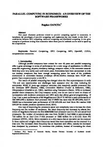
numerical realization and can not be used for a deep analysis without additional procedures. On the Fig.1 one can see two levels of the simulation process using the tracking method. The inner level admits parallelization procedure naturally. The outer level has sequential character and usually can not be realized on parallel computers (see the Fig.1).
2.2
where Hk = Hk X [k] , Vk = Vk X [k] are homogeneous polynomials of k -th order. The matrices H k or Vk can be calculated with the help of the continuous analogue of the CBH-and Zassenhauss formulae and by using the Kronecker product and Kronecker sum technique for matrices [7]. Moreover, using the matrix representation for the Lie operators one can write a matrix representation for the Lie map generated by these Lie operators
M 1 M10 M11 M12 M1
The Mapping Method
M�X =
This method is based on the priority of map creation. Using a database of accelerator elements (drifts, dipoles, multipole lenses and so on) we computer a map generated by the machine. In this case an accelerator or its part are described as a dynamical system with control. In this work we use the matrix formalism for Lie algebraic methods developed in previous works [7]–[9].
= (
dX ds
(1)
= F (X; U; s)
a motion equation for beam particles in external and spacecharge fields. Here the vector U (s) describes control functions corresponding to guiding and focusing fields. Any solution of this equation can be written in the form X (s) = M(sjs0 ) � X0 ;
X0 2
M
0;
where M(sjs0 ) is so called Lie map (transformation). This map satisfies to the following operator equation M(sjs0 )(s) = LF � M(sjs0 );
M(s0 js0 ) = I d;
where LF is a Lie operator associated with the function F from the Eq.(1). For non-autonomous systems the so called Magnus’s representation [7] is used. This approach allows to pass from the time-ordered exponent operator to a routine exponential operator. The expansion of the function F (X; s): F (X; s) =
1 X
P1
k
(s)X
[k ]
k=0
generates P 1 G
an expansion of the function G(X ; tjt 0 ) = [k ] which appears in the Magnus’s rep(tjt0 )X k k=0 resentation and one can write M(tjt0 ) = exp
(X 1 k=0
Gk (X; U ; tjt0 ) =
G
)
j
LG (X;U ;t t0 ) k
k (U ; tjt0 ) X
[k ]
;
:
The similar to the Dragt-Finn factorization for the Lie transformations allows to rewrite the exponential operator as an infinite product of exponential operators of Lie operators M = : : : � expfLH2 g � expfLH1 g = = expfLV1 g � expfLV2 g � : : : ;
1352
k
:::
=
1 X
M1
k
X
[k]
=
: : :)X
1= (2)
;
k=0
X
The Lie Algebraic Tools. Let be
X
1 = (1 X X [2] : : : X [
k]
�
: : :) ;
where the matrices M1k (solution matrices) can be calculated according to the recurrent sequence of formulae of the following types: Mk � X
= X
[l]
+
1 X m=1
1 m!
[l]
= expfLGk g � X
Y m
G�((
j
m
1)(k
[l]
1)+l)
=
X
[m(k
1)+l]
;
j =1
where G�l = G�(l 1) E + E[l 1] G denotes the Kronecker sum of l-th order. For the inverse map M 1 : 1 X ! X0 = M � X one can compute the corresponding block-matrices using the generalized Gauss’s algorithm. Computer Algebra and Knowledge Bases. The desired solution is created in the form of power series. It is clear that this way can be realized only with truncated procedures for some chosen order of expansions – the approximation order N . In the referred works the corresponding matrices P1k , Gk , Hk , Vk and M1k are calculated up to seventh order in symbolic forms using the computer algebra codes (MAPLE V). These tools have algebraic character and can be easily realized on parallel computers. The Map Creation. Knowledge of the Lie map in the matrix form (see the Eq.(2)) up to some approximation order N allows to create necessary criteria for beam line working and current images (s) = M(sjs0 ) � 0 . We should note that the approximation order N has to make consistent with the order of approximation for the external and space charge fields. In this approach one follows current phase beam portraits. These portraits allow to calculate additional criteria of beam evolution. From computing point of view this approach has two levels of realization too. But in contrast to the tracking method the mapping method has another structure of computational process (see the Fig.2). The map computing (the inner level) is based on a set of ready matrices M1k (sjs0 ) for different accelerator elements calculated in symbolic forms (using computer algebra codes REDUCE M(sjs0 )
M
M
Proceedings of EPAC 2000, Vienna, Austria
The Advantage of the Mapping Method. From computing point of view the second approach based on the mapping method is more preferable. Indeed at first we have two parallel processes: for maps computation and for phase portraits computation. In the second we can use the prepared in advance matrices 1k (extracting them from the corresponding database). From analytical point of view the mapping method is also preferable as one can analyze corresponding criteria without beam images calculation.
M
3
Figure 1: The calculation scheme according to the tracking method. There two levels of calculations: the inner level I is based on the motion equations solver. The initial data flow realizes the computing beam phase portraits on the outer level II.
CONCLUSION
The discussed approaches is verified on some test problems (for example, for halo formation process). For some models of beam lines we approved these approaches on the base of the High Performance Center of St.-Petersburg State University. These computer experiments confirmed our estimates of effectiveness of these approaches.
REFERENCES [1] J. A. Holmes, V. V. Danilov, J. D. Galambos, D. Jeon, and D. K. Olsen, Phys.Rev.Special Topics - Accel.and Beams, 2, 114202, 1999. [2] J. Qiangy ,R. D. Ryne, S. Habib, Proc. of the 1999 Particle Accelerator Conference, N.Y., (1999), pp.366–368. [3] Tai-Sen F. Wang and Thomas P. Wangler, Proc. of the 1999 Particle Accelerator Conference, N.Y., (1999),pp.1848– 1850. [4] S.N. Andrianov, A.I. Dvoeglazov, Proc. of the 1997 Particle Accelerator Conference, Vancouver, BC, Canada, 1997, pp.2419–2421. [5] S.N. Andrianov, A.I. Dvoeglazov, Proc. of the Sixth European Particle Accelerator Conference, Stockholm, Institute of Physics Publishing, Bristol, UK, pp.1150–1152.
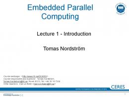
Figure 2: The calculation scheme according to the mapping method. There two levels of calculations: the inner level I is based on the map calculation in the matrix forms. This process has a parallel character as it is based on the matrix algebra. The initial data flow enters on the outer level II.
[6] A.J. Dragt, Physics of High Energy Particle Accelerators. Eds. Carrigan, Huson F.R., Month M. AIP Conf. Proc., 87, NY, 1982, pp.147–313.
and MAPLE V). These matrices are the fulfilment of the corresponding database. It is known that the matrix algebra admits the parallelization in a natural way. Then one can calculate necessary criteria using only matrix elements of current matrices 1k , k � N (see, for example, [10]). On the outer level we i=use the beam information in the different forms: 1) the model initial distribution function f0 (X ), X 2 0 [10]; 2) the equipotential surfaces or lines for the� initial phase portrait 0 presentation: G0 (X ) = C , 1 m , where m is the number of levels; 3) the C = g0 ; : : : ; g0 pointwise presentation of the 0 . This information treat in to the calculation process for those sections for which one wants to study the beam behaviour. So we deal with the so called MIMD (Multiple Instruction, Multiple Data) technology.
[8] S.N. Andrianov, Proc. of the Second Int.Workshop Beam Dynamics & Optimization, 1995, St.Petersburg, Russia, SPbSU, St.Petersburg, 1996, pp.25–32.
M
M
[7] S.N. Andrianov, Proc. of the 1996 Computational Accelerator Physics Conference – CAP’96, Sept. 24–27, Williamsburg, Virginia, USA, eds. J.J.Bisognano, A.A.Mondelli, AIP Conf. Proc. 391, NY, 1997, pp.355–360.
[9] S.N.Andrianov, Proc. of the Sixth European Particle Accelerator Conference, Stockholm,1998, Institute of Physics Publishing, Bristol, UK, pp.1091–1093. [10] S.N.Andrianov, V.M.Taryanik, in this Proc.
M M
Proceedings of EPAC 2000, Vienna, Austria
1353