Parallel Computing With Cuda in Image Processing

Parallel Computing With Cuda in Image Processing corrado ameli 1 12 October 2017

contents 1 2 3 4 5

6

Introduction State Of The Art Nvidia CUDA 3.1 Workflow . . . . . . . . . . . . . . . . . . . . Methodology Loading and Gathering 5.1 CPU Loading Time . . . . . . . . . . . . . . 5.2 GPU Loading and Gathering Time . . . . . 5.3 Overall Timing . . . . . . . . . . . . . . . . Image Processing Functions 6.1 Binary Image Distance Transform . . . . . 6.2 Binary Image Labeling . . . . . . . . . . . . 6.3 Binary Image Filtering with Lookup Tables 6.4 Binary Morphological Operations . . . . . 6.5 Image Correlation . . . . . . . . . . . . . . . 6.6 Edge Detection . . . . . . . . . . . . . . . . 6.7 Histogram Equalization . . . . . . . . . . . 6.8 Image Absolute Difference . . . . . . . . . . 6.9 Image Contrast Enhancement . . . . . . . . 6.10 Image Top-Hat and Bottom-Hat Filtering . 6.11 Image Morphological Closing . . . . . . . . 6.12 Image Complement . . . . . . . . . . . . . . 6.13 Image Dilation . . . . . . . . . . . . . . . . . 6.14 Image Erosion . . . . . . . . . . . . . . . . . 6.15 Image Filling . . . . . . . . . . . . . . . . . . 6.16 Image Filtering . . . . . . . . . . . . . . . . 6.17 Image Gaussian Filtering . . . . . . . . . . . 6.18 Image Gradient . . . . . . . . . . . . . . . . 6.19 Image Histogram . . . . . . . . . . . . . . . 6.20 Linear Image Combination . . . . . . . . . 6.21 Image Morphological Opening . . . . . . . 6.22 Image Morphological Reconstruction . . . 6.23 Displacement Field Estimation . . . . . . . 6.24 Image Resize . . . . . . . . . . . . . . . . . . 6.25 Image Rotation . . . . . . . . . . . . . . . . 6.26 Median Filtering . . . . . . . . . . . . . . . 6.27 Standard Deviation Filtering . . . . . . . .

. . . . . . . . . . . . . . . .

. . . . . . . . . . . . . . . . . . . . . . . . . . . . . . . . . . . . . . . . . . . . . . . . . . . . . . . . . . . . . . . . . . . . . . . . . . .

. . . . . . . . . . . . . . . . . . . . . . . . . . .

. . . . . . . . . . . . . . . . . . . . . . . . . . .

. . . . . . . . . . . . . . . . . . . . . . . . . . .

. . . . . . . . . . . . . . . . . . . . . . . . . . .

. . . . . . . . . . . . . . . . . . . . . . . . . . .

. . . . . . . . . . . . . . . . . . . . . . . . . . .

. . . . . . . . . . . . . . . . . . . . . . . . . . .

. . . . . . . . . . . . . . . . . . . . . . . . . . .

. . . . . . . . . . . . . . . . . . . . . . . . . . .

. . . . . . . . . . . . . . . . . . . . . . . . . . .

. . . . . . . . . . . . . . . . . . . . . . . . . . .

. . . . . . . . . . . . . . . . . . . . . . . . . . .

. . . . . . . . . . . . . . . . . . . . . . . . . . .

. . . . . . . . . . . . . . . . . . . . . . . . . . .

. . . . . . . . . . . . . . . . . . . . . . . . . . .

4 4 4 5 5 6 6 6 7 7 7 8 8 8 8 9 9 9 10 11 11 12 12 13 13 13 14 14 14 15 15 16 16 17 17 17 18

1

List of Figures Scenarios 7.1 Scenario 1 . . . . . . . . . . . 7.2 Scenario 2 . . . . . . . . . . . 8 Conclusion 8.1 Gain Analysis . . . . . . . . . 8.2 Standard Deviation Analysis 9 Hardware Configuration 10 Figures 11 References 7

. . . . . . . . . . . . . . . . . . . . . . . . . . . . . . . . . . . . . . . . . . . . . . . . . . . . . . . . . . . . . . . . . . . . . . . . . . . . . . . . . . . . . . . . . . . . . . . .

19 19 20 22 22 22 23 24 35

list of figures Figure 1 Figure 2 Figure 3 Figure 4 Figure 5 Figure 6 Figure 7 Figure 8 Figure 9 Figure 10 Figure 11 Figure 12 Figure 13 Figure 14 Figure 15 Figure 16 Figure 17 Figure 18 Figure 19 Figure 20 Figure 21 Figure 22 Figure 23 Figure 24 Figure 25 Figure 26 Figure 27 Figure 28

Nvidia CUDA Workflow . . . . . . . . . . . Nvidia CUDA Hierarchy . . . . . . . . . . . CPU vs GPU Loading Comparison. . . . . Binary Image Distance Transorm Example Binary Labeling Example . . . . . . . . . . Binary Filtering with LUT Example . . . . Binary Morphological Filtering . . . . . . . Histogram Equalization . . . . . . . . . . . Image Absolute Difference . . . . . . . . . . Image Contrast Enhancement . . . . . . . . Top Hat Filtering . . . . . . . . . . . . . . . Image Morphological Closing . . . . . . . . Image Dilation . . . . . . . . . . . . . . . . . Image Filling . . . . . . . . . . . . . . . . . . Linear Combination . . . . . . . . . . . . . . Morphological Opening . . . . . . . . . . . Morphological Reconstruction . . . . . . . . Displacement Field Estimation . . . . . . . Median Filtering . . . . . . . . . . . . . . . . Standard Deviation Filtering . . . . . . . . . Scenario 1 - Aerial Photo . . . . . . . . . . . Scenario 1 - Thresholded Photo . . . . . . . Scenario 1 - Highlighted Photo . . . . . . . Scenario 2 - Raw Image . . . . . . . . . . . . Scenario 2 - Gradient Magnitude Photo . . Scenario 2 - Foreground Marking Photo . . Scenario 2 - Background Marking Photo . . Scenario 2 - Segmented Photo . . . . . . . .

. . . . . . . . . . . . . . . . . . . . . . . . . . . .

. . . . . . . . . . . . . . . . . . . . . . . . . . . .

. . . . . . . . . . . . . . . . . . . . . . . . . . . .

. . . . . . . . . . . . . . . . . . . . . . . . . . . .

. . . . . . . . . . . . . . . . . . . . . . . . . . . .

. . . . . . . . . . . . . . . . . . . . . . . . . . . .

. . . . . . . . . . . . . . . . . . . . . . . . . . . .

. . . . . . . . . . . . . . . . . . . . . . . . . . . .

. . . . . . . . . . . . . . . . . . . . . . . . . . . .

. . . . . . . . . . . . . . . . . . . . . . . . . . . .

. . . . . . . . . . . . . . . . . . . . . . . . . . . .

24 25 25 26 26 26 27 27 27 28 28 28 29 29 29 29 30 30 30 30 31 31 32 32 33 33 34 34

Table of Image Sizes . . . . . . . . . . . . . . . . . CPU Loading Time . . . . . . . . . . . . . . . . . . GPU Loading and Gathering Time . . . . . . . . . Overall Overhead Introduced By GPU Migration . BIDT Comparison . . . . . . . . . . . . . . . . . . . Binary Labeling Comparison . . . . . . . . . . . . Binary LUT Filtering Comparison . . . . . . . . . Binary Morphological Filtering Comparison . . . Image Correlation Comparison . . . . . . . . . . . Edge Correlation Comparison . . . . . . . . . . . .

. . . . . . . . . .

. . . . . . . . . .

. . . . . . . . . .

. . . . . . . . . .

. . . . . . . . . .

. . . . . . . . . .

. . . . . . . . . .

6 6 6 7 7 8 8 9 9 10

list of tables Table 1 Table 2 Table 3 Table 4 Table 5 Table 6 Table 7 Table 8 Table 9 Table 10

2

List of Tables Table 11 Table 12 Table 13 Table 14 Table 15 Table 16 Table 17 Table 18 Table 19 Table 20 Table 21 Table 22 Table 23 Table 24 Table 25 Table 26 Table 27 Table 28 Table 29 Table 30 Table 31 Table 32 Table 33

Histogram Equalization Comparison . . . . . . . . Image Absolute Difference Comparison . . . . . . Image Absolute Difference Comparison . . . . . . Top-Hat and Bottom-Hat Filtering Comparison . . Image Morphological Closing Comparison . . . . Image Complement Comparison . . . . . . . . . . Image Dilation Comparison . . . . . . . . . . . . . Image Erosion Comparison . . . . . . . . . . . . . Image Filling Comparison . . . . . . . . . . . . . . Image Filtering Comparison . . . . . . . . . . . . . Image Gaussian Filtering Comparison . . . . . . . Image Gradient Comparison . . . . . . . . . . . . Image Histogram Comparison . . . . . . . . . . . Linear Image Combination Comparison . . . . . . Image Morphological Opening Comparison . . . Image Morphological Reconstruction Comparison Displacement Field Estimation Comparison . . . . Image Resize Comparison . . . . . . . . . . . . . . Image Rotation Comparison . . . . . . . . . . . . . Median Filtering Comparison . . . . . . . . . . . . Standard Deviation Filtering Comparison . . . . . Scenario 1 Comparison . . . . . . . . . . . . . . . . Scenario 2 Comparison . . . . . . . . . . . . . . . .

. . . . . . . . . . . . . . . . . . . . . . .

. . . . . . . . . . . . . . . . . . . . . . .

. . . . . . . . . . . . . . . . . . . . . . .

. . . . . . . . . . . . . . . . . . . . . . .

. . . . . . . . . . . . . . . . . . . . . . .

. . . . . . . . . . . . . . . . . . . . . . .

. . . . . . . . . . . . . . . . . . . . . . .

10 11 11 11 12 12 12 13 13 14 14 15 16 16 16 17 17 17 18 18 18 19 22

abstract This report is intended to give a broad perspective on the use of parallel computing in image processing, focusing on the most recent technology developed by Nvidia: CUDA. Through a quantitative analysis in Matlab environment, the differences between standard computation (CPU) and parallel computation will be highlighted. In order to achieve this, several scenarios of classic image processing and processing techniques will lead this report.

1

Department of Informatics, University of Milan, Crema, Italy

3

introduction

1

introduction

The demand of real-time high-resolution 2D and 3D processing is continuously growing since the birth of Computer Vision. The hardware nature of a Graphic Processing Unit (GPU), composed by thousands of basic operations cores, can be exploited to perform certain kinds of operation several times faster. Most of the algorithms working with matrices (like images) are likely to be parallelized, due to the nature of the data itself. The gain achieved by moving the computation from the CPU to the GPU can vary significantly depending on the nature of the image (binary, greyscale, color), on the resolution of the image and on the implementation of the algorithm. Matlab offers a wide variety of Image Processing functions implemented in both serial and parallel way, which makes it a good environment for testing the potential of this alternative kind of computation. Moreover, Matlab has embedded an interface to CUDA which allows the user to use high technology parallel architectures in a very transparent way, which yields to an easy and clean programming approach. Through a quantitative analysis of image processing techniques, and through the simulation of scenarios, an overview of the temporal advantages that can be achieved through CUDA parallelization is presented.

2

state of the art

During the last decade, parallel computing has become a very discussed topic, even if the very first approaches to GPU computation were made in the 80s [1]. Works from the beginning of the century like [2], acclaimed this computation as the new "era" of technology, finding patterns [3] to distinguish whether an application may present some gain with parallelization. Several articles on GPGPU (General Purpose GPU) performance evaluation and design have been proposed in literature [4][5][6]. Two similar works [7][8] in image processing were proposed a decade ago. A good introduction to CUDA (summarized in Section 3) is presented in this work[9]. Nowadays, Parallel Image Processing is used in several fields such as Medical Analysis [10][11][12], near-field localization [13][14], facial recognition [15][?] and many others. The development of CUDA has become a focus on academic researches. People not only use CUDA to deal with graphics and images, but also use it to handle numerical calculations. For example, R. R. Amossen et al. reported a novel data layout called BATMAP, suitable for parallel processing, which is compact even for sparse data [16]. This work [17] described an automated compilation flow that maps most stream processing applications onto GPUs by taking important architectural features of NVIDIA GPUs into consideration. Grand et al. proposed a broad-phase collision detection with CUDA [18]. A. A. Aqrawi et al. presented a method using compression for large seismic data sets on modern GPUs and CPUs [19]. Later, A. A. Aqrawi et al. presented the 3D convolution for large data sets on modern GPUs [20]. J. Barnat et al. designed a new CUDA-aware procedure for pivot selection and implemented parallel algorithms using CUDA accelerated computation [21].

3

nvidia cuda

Nvidia CUDA is a platform designed to offer general purpose processing with CUDA-enabled GPUs. CUDA offers a layer which allows the programmer to directly use a virtual instruction set in order to perform operations on the device.

4

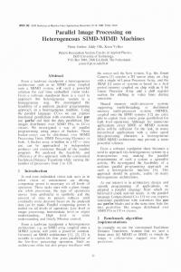
methodology CUDA has a complex hierarchical structure, which is intended to maximize the efficiency of the hardware. An application is divided in serial portions. Each portion may be parallelized. The portions that can actually be parallelized are executed as a kernel. Several kernels can be executed at once. Each kernel launches thousands of threads and groups them into grids. Grids are an abstract level of block grouping which work is common. Blocks are groups of threads which are linked to a particular group of cores called Streaming Multiprocessors. This complex hierarchy is used to achieve different levels of parallelism and memory sharing among different layers, providing efficiency and scalability. A scheme of the complete hierarchy is presented in Figure 2 on page 25. Moreover, a kernel can actually specify to launch more threads than the GPU can handle concurrently in order to amortize the throughput time. 3.1 Workflow As shown in Figure 1 on page 24, the workflow of a typical scenario consists of 4 steps: 1. Copy processing data 2. Instruct the processing 3. Execute parallel in each core 4. Copy the result Firstly, the processing data is copied from the Main Memory (RAM) to the GPU Memory. This means that the data cannot be directly loaded into the GPU except for very standard ones (e.g. empty matrices) of which the GPU instruction set is capable of locally allocate. From CUDA version 6.0+ a new improvement has been introduced called Unified Memory. Unified Memory hides the fact that CPU memory and GPU memory are physically separated: programming becomes easier and performance increases because of how CUDA migrates the data using asynchronous streams. Once the data is copied, the CPU instructs the process to the GPU about the computation to be off loaded. The computation can now begin. CUDA devices also offer shared memory among threads which acts as a cache which is roughly 100x faster than global memory. Lastly, the results are gathered and copied back to the Main Memory. As the reader may realize, the loading and gathering time could be critical to determine whether the parallel computing could outstand the CPU. In the following chapter, this aspect is analyzed.

4

methodology

All the images considered are PNG files with 32 bit depth and all the evaluations are performed over 1000 iterations of the same operation except for Scenario 2 ( 7.2 ) which has been evaluated over 100 iterations. In order to measure performance in Matlab, tic and toc functions have been used. The time gathered is approximated to microseconds (1 ∗ 10−6 ). In Section 6 and 7, the column Gain is evaluated as: ((meancpu /meangpu ) − 1) ∗ 100

For instance, if GPU and CPU achieve the same result, then the gain is 0. If GPU computation is 2x faster than CPU, the gain is 100%.

5

loading and gathering The images used in Section 6 are scaled in several common sizes listed in Table 1. Some of the tests performed in Section 6 were not successful because of CUDA errors which nature was unspecified. The technical support of NVIDIA was not able to solve this problem in short terms. Table 1: Table of Image Sizes

5

N.

Format

Width

Height

Size

1 2 3 4 5 6 7

360p 480p 720p 2K 4K 8K 16K

640 854 1280 1920 3840 7680 15360

360 480 720 1080 2160 4320 8640

354 KB 573 KB 1.09 MB 2.87 MB 4.78 MB 15.0 MB 42.0 MB

loading and gathering

Firstly, the loading time of the Main Memory will be analyzed, followed by a sum up of time needed to migrate the data to the GPU memory and to gather it back. 5.1 CPU Loading Time

Table 2: CPU Loading Time

N.

Format

Average (s)

Size

Avg. Transfer Speed (MBps)

1 2 3 4 5 6 7

360p 480p 720p 2K 4K 8K 16K

0.0097 0.0163 0.032 0.0881 0.1894 0.6986 2.5616

354 KB 573 KB 1.09 MB 2.87 MB 4.78 MB 15.0 MB 42.0 MB

36.494 35.153 34.062 32.576 25.237 21.471 16.396

As it can be observed in Table 2, the average transfer speed of small images in the Main Memory is higher. This is good for real-time general purpose image processing where the data is usually small sized. 5.2

GPU Loading and Gathering Time

Table 3: GPU Loading and Gathering Time N.

Format

Loading Avg (s)

Gathering Avg (s)

ALS (MBps)

AGS (MBps)

1 2 3 4 5 6 7

360p 480p 720p 2K 4K 8K 16K

0.0021 0.0004 0.0009 0.0015 0.0057 0.0204 0.0756

0.0003 0.0008 0.0014 0.0029 0.0122 0.055 0.1821

168.571 1.432.500 1.211.000 1.913.333 838.596 735.294 555.555

1.180.000 716.250 778.571 989.655 391.803 272.727 230.642

6

image processing functions Table 3 on the preceding page shows that the average loading speed (ALS) and the average gathering speed (AGS) are several times faster than the ATS of the Main Memory shown in Table 2 on the previous page. In this case, the speed is not proportional to the size of the data, probably because for small files the time needed for management of the transfer is higher than the actual migration of the data itself. 5.3 Overall Timing In Figure 3 on page 25 an overview of the collected data is presented. The overhead introduce by the migration of the data is shown in Table 4. With respect to the loading time of the Main Memory, the migration of the data to the GPU increases by approximately less than 10% the overall time. In the following sections, this data will be taken into account in order to understand if the delay introduced by the migration is worth compared to the temporal advantages achieved with parallel computing. Table 4: Overall Overhead Introduced By GPU Migration

6

N.

Format

L. CPU Avg

L. GPU Avg

G. GPU Avg

Total

Overhead

1 2 3 4 5 6 7

360p 480p 720p 2K 4K 8K 16K

0.0097 0.0163 0.032 0.0881 0.1894 0.6986 2.5616

0.0021 0.0004 0.0009 0.0015 0.0057 0.0204 0.0756

0.0003 0.0008 0.0014 0.0029 0.0122 0.055 0.1821

0.0121 0.0175 0.0343 0.0925 0.2073 0.774 2.8193

24% 7.36% 7.18% 4.99% 9.45% 10.79% 10.06%

image processing functions

In this section each function contained into the Image Processing Toolkit provided by MATLAB that supports parallelism is analyzed. 6.1 Binary Image Distance Transform The Distance Transform of a binary image is a map that assigns to each pixel the distance to the closest black pixel. The distance can be calculated with several methods depending on the level of edge smoothness that needs to be achieved. A common use of BIDT is to smooth the image once a binary threshold has been applied as shown in Figure 4 on page 26. Table 5: BIDT Comparison

N.

Format

CPU Avg (s)

GPU Avg (s)

Gain (%)

1 2 3 4 5 6

360p 480p 720p 2K 4K 8K

0.0020 0.004 0.008 0.0239 0.0921 0.3986

0.00007 0.0002 0.0004 0.0012 0.0048 0.0213

2757 % 1900 % 1900 % 1800 % 1800 % 1775 %

In Table 5 the average running times are presented. GPU outstands with a 17/20+ times faster computation than CPU.

7

image processing functions 6.2 Binary Image Labeling Binary Labeling allows to label connected components in 2D images. It is commonly used to find separated objects in space like in Figure 5 on page 26 once the image has been binarized. Different colors in the image represents different labels. Table 6: Binary Labeling Comparison

N.

Format

CPU Avg (s)

GPU Avg (s)

Gain (%)

1 2 3 4 5 6

360p 480p 720p 2K 4K 8K

0.0014 0.0024 0.0047 0.0095 0.0305 0.1088

0.0026 0.0032 0.0043 0.0068 0.0194 0.0686

-46% -25% 11% 28% 36% 37%

The Table 6 shows how with small image resolutions CPU is faster, while starting from 720p, GPU offers a moderate speed up. 6.3 Binary Image Filtering with Lookup Tables This filtering technique is achieved by using Lookup Tables (LUT). There is one LUT for each pixel and its entries contain the binary value of the 9 neighbors. By defining a function that expresses the new value of the single pixel from the values of the neighbors, several types of filters can be produced. For instance, in Figure 6 on page 26 a erosion of the edges is performed by using a function that returns 1 (white pixel) iif the sum of the neighbors is at least 4. As a result, the text in the image becomes thinner. Table 7: Binary LUT Filtering Comparison

N.

Format

CPU Avg (s)

GPU Avg (s)

Gain (%)

1 2 3 4 5 6

360p 480p 720p 2K 4K 8K

0.0006 0.0009 0.0019 0.0042 0.0162 0.0666

0.0022 0.025 0.0033 0.0051 0.0181 0.0627

-72% -64% -42% -17% -10% 6%

From Table 7 we can see how GPU does not produce good results compared to CPU computation especially on low resolution images. 6.4 Binary Morphological Operations In MATLab, the function bwmorph allows the user to use predefined matrices as filters to be convoluted with the image itself. In this subsection we are going to use the remove option which produces a filtering operation like in Figure 7 on page 27 where only the edges of the figure become visible. As reported in Table 8 on the next page, it is obvious how GPU outstands in operations like convolution which, by nature, are more likely to be parallelized. 6.5 Image Correlation Image correlation compares two images and returns their level of similarity. Two identical images have 100% correlation. For this analysis, a comparison between

8


Table 8: Binary Morphological Filtering Comparison

N.

Format

CPU Avg (s)

GPU Avg (s)

Gain (%)

1 2 3 4 5 6

360p 480p 720p 2K 4K 8K

0.0004 0.0005 0.0011 0.0024 0.01 0.035

0.0002 0.0002 0.0002 0.0003 0.0004 0.0004

100% 150% 450% 600% 2400% 8650%

two copies of a picture have been taken into account, one of them is noised with random grains by using imnoise function by MATLab. Table 9: Image Correlation Comparison

N.

Format

CPU Avg (s)

GPU Avg (s)

Gain (%)

1 2 3 4 5 6

360p 480p 720p 2K 4K 8K

0.0035 0.0058 0.0131 0.0297 0.0385 0.837

0.0032 0.0033 0.0039 0.0051 0.0057 0.0085

9% 75% 235% 482% 575% 884%

As shown in Table 9, GPU achieves great results as long as the image resolution grows. 6.6 Edge Detection Edge Detection can be achieved with several methods like Prewitt, Roberts, Laplacian of Gaussian, Sobel or Canny (not supported on GPU). In Table 10 on the next page, we can see that Sobel and Prewitt methods have quite similar trends. With a small resolution of 360p, CPU still computes faster, but further on GPU achieves a better performance. With Roberts method, GPU still performs better. Finally, with LOG method, GPU has optimal performance, achieving a 15/20 times faster computation. 6.7

Histogram Equalization

Histogram Equalization (HE) is a contrast enhancer. HE models the image as a probability density function and seeks to make equiprobable the probability for a pixel to take on a particular intensity. An example of HE is shown in Figure 8 on page 27 where the wheel has more visible details once the function is performed. In Table 11 on the next page, we can see how CPU performs better in most of the cases, thus the parallelized version of HE shall be used only with high resolution datatypes. 6.8

Image Absolute Difference

Image Difference is a common operation that can be used in several scenarios. It can be used to locate regions of dissimilarity on slightly different images or to remove objects or background once the target has been identified. In Figure 9 on page 27 we can see how image difference can be used for instance to highlight common areas among different objects in the same space.

9


Table 10: Edge Correlation Comparison

Method

Sobel

Prewitt

Roberts

LOG

N.

Format

CPU Avg (s)

GPU Avg (s)

Gain (%)

1 2 3 4 5 6

360p 480p 720p 2K 4K 8K

0.0020 0.0038 0.0087 0.0197 0.08 0.4138

0.0024 0.0028 0.0040 0.0063 0.018 0.2610

-20% 36% 117% 212% 344% 58%

1 2 3 4 5 6

360p 480p 720p 2K 4K 8K

0.0019 0.0041 0.0086 0.0189 0.0768 0.4022

0.0023 0.0029 0.0040 0.0063 0.0181 0.2809

-21% 41% 115% 200% 324% 43%

1 2 3 4 5 6

360p 480p 720p 2K 4K 8K

0.0032 0.0060 0.0126 0.0288 0.1046 0.4504

0.0027 0.0029 0.0035 0.0054 0.0164 0.4071

18% 106% 160% 430% 537% 10%

1 2 3 4 5 6

360p 480p 720p 2K 4K 8K

0.0091 0.0232 0.0512 0.1211 0.4904 1.9041

0.0037 0.0043 0.0055 0.0085 0.0243 0.1137

145% 439% 830% 1324% 1900% 1500%

In Table 12 on the next page, the data shows that GPU computation outstands only with very high resolutions while CPU performs better in most of the common configurations. 6.9 Image Contrast Enhancement Image Contrast Enhancement is achieved by normalizing the intensity scale of an image in a particular range. For instance, if an image has a low contrast and presents important data (like objects we want to observe) in the range of a greyscale 100-120, this technique will normalize the 100 gradient as a 0 and the 120 gradient as a 255. If this technique is used with a range equal to the bounds of the intensity scale of the image, the intensity components are normalized through the whole grey or rgb spectrum, achieving a better contrast.

Table 11: Histogram Equalization Comparison

N.

Format

CPU Avg (s)

GPU Avg (s)

Gain (%)

1 2 3 4 5 6

360p 480p 720p 2K 4K 8K

0.0006 0.0008 0.0014 0.0020 0.0060 0.0225

0.0014 0.0015 0.0018 0.0025 0.0.0052 0.0153

-58% -47% -33% -20% 15% 47%

10


Table 12: Image Absolute Difference Comparison

N.

Format

CPU Avg (s)

GPU Avg (s)

Gain (%)

1 2 3 4 5 6

360p 480p 720p 2K 4K 8K

0.00007 0.0001 0.00013 0.002 0.0023 0.0092

0.00015 0.00017 0.00018 0.0025 0.0.00026 0.00035

-114% -70% -38% -25% 784% 2520%

In Figure 10 on page 28 an example of Image Contrast Enhancement is presented, where a big improvement of the contrast is visible with naked eyes. Table 13: Image Absolute Difference Comparison

N.

Format

CPU Avg (s)

GPU Avg (s)

Gain (%)

1 2 3 4 5 6

360p 480p 720p 2K 4K 8K

0.0011 0.0015 0.0030 0.0072 0.0026 0.1

0.0043 0.0044 0.0053 0.0074 0.0.0018 0.06

-300% -193% -76% -2% 44% 66%

In Table 13, GPU performs slightly better only on very high resolutions, while CPU scores better in mid and low resolutions. 6.10 Image Top-Hat and Bottom-Hat Filtering The top-hat filter is used to enhance bright objects of interest in a dark background. The bottom-hat filter is used to do the opposite. The filters work by suppressing large regions while keeping the small ones, as specified by the size of a structuring element provided by the user. In Figure?? a top-hat filtering has been applied by specifying a disk of a determined radius as a structuring element. The main big blob is thus deleted from the image, preserving all the small blobs. In Table 14 the results of both the filters are presented. Parallel computation is several times faster as the resolution grows compared to standard computation. Table 14: Top-Hat and Bottom-Hat Filtering Comparison

N.

Format

CPU Avg (s)

GPU Avg (s)

Gain (%)

1 2 3 4 5 6

360p 480p 720p 2K 4K 8K

0.0068 0.0096 0.0145 0.0357 0.1292 0.5146

0.0033 0.0035 0.0035 0.0035 0.0039 0.0045

106% 174% 314% 902% 3200% 11300%

6.11 Image Morphological Closing Image Morphological Closing is a mix of dilation and erosion performed with the usage of a structuring element given by the user. Basically the structuring element reshapes the outline of the image and, if big enough, fills the inside. An example is presented in Figure 12 on page 28 where the figure becomes fully white filled.

11


Table 15: Image Morphological Closing Comparison

N.

Format

CPU Avg (s)

GPU Avg (s)

Gain (%)

1 2 3 4 5 6

360p 480p 720p 2K 4K 8K

0.0070 0.0093 0.0144 0.0380 0.1369 0.5260

0.0033 0.0033 0.0034 0.0036 0.0.0040 0.0043

112% 181% 323% 905% 3323% 12100%

Like all the previous morphological operations, GPU performs several times faster as shown in Table 15. 6.12 Image Complement Image Complement is obtained by subtracting from each pixel the maximum pixel value supported by the class. Table 16: Image Complement Comparison

N.

Format

CPU Avg (s)

GPU Avg (s)

Gain (%)

1 2 3 4 5 6

360p 480p 720p 2K 4K 8K

0.00009 0.0003 0.0006 0.0014 0.006 0.0252

0.00009 0.0001 0.0001 0.0001 0.0.0002 0.0002

0% 200% 500% 1300% 2900% 12500%

In 16 the data presented shows how this simple operation is performed much better with GPU. 6.13 Image Dilation Image Dilation dilates the binary or greyscale objects in the image with respect to a structuring element defined by the user. An example of Image Dilation with a binary source is shown in Figure 13 on page 29, where the structuring element is a vertical line. As a result, the text becomes dilated vertically and while the upper text remains legible, the lower one becomes unreadable. Table 17: Image Dilation Comparison

N.

Format

CPU Avg (s)

GPU Avg (s)

Gain (%)

1 2 3 4 5 6

360p 480p 720p 2K 4K 8K

0.0031 0.0039 0.0061 0.016 0.0578 0.2216

0.0029 0.0019 0.0019 0.0022 0.0024 0.0026

8% 108% 215% 639% 2969% 8374%

The results contained in Table 17 show a good score of GPU computation, that grows higher as the resolution increases.

12

image processing functions 6.14 Image Erosion Image Erosion is the counterpart of Image Dilation. Thus, the user-defined structuring element is used to erode the image with respect to the greyscale intensity of the area. Table 18: Image Erosion Comparison

N.

Format

CPU Avg (s)

GPU Avg (s)

Gain (%)

1 2 3 4 5 6

360p 480p 720p 2K 4K 8K

0.0028 0.0037 0.0057 0.0151 0.0551 0.2164

0.0015 0.0015 0.0016 0.0017 0.0020 0.0022

90% 146% 263% 784% 2646% 9657%

The results presented in Table 18 are similar to the results shown in the previous subsection. Thus, Image Erosion and Image Dilation share the same gain of performance. 6.15 Image Filling Image Filling is a technique that works differently if the input is either a binary image or a greyscale image. In a binary image, Image Filling fills all the 0 areas surrounded by 1, starting from a point specified by the user. In a greyscale image, a hole is defined as an area of dark pixels surrounded by lighter pixels. Thus, the function fills the areas surrounded either by lighter or darker pixels. An example of greyscale image filling is presented in Figure 14 on page 29 where the three main parts of the wheel are distinguished. Table 19: Image Filling Comparison

N.

Format

CPU Avg (s)

GPU Avg (s)

Gain (%)

1 2 3 4 5 6

360p 480p 720p 2K 4K 8K

0.0072 0.0144 0.0317 0.0751 0.2302 1.0992

0.0228 0.0274 0.0431 0.0662 0.1365 -

-215% -90% -36% 13% 68% -

From Table 19 we can assert that the parallelized implementation is not efficient with low resolutions. Furthermore, 8K test was not supported by CUDA, returning an unspecified launch failure. 6.16 Image Filtering Image Filtering can be achieved through two mathematical operators: correlation and convolution. The desired filter can be obtained by using the function fspecial. Correlation and convolution options share the same performance both in GPU and CPU computation. GPU performance shows its best in filtering as shown in Table 20 on the next page achieving from 3 to 37 times faster computation.

13


Table 20: Image Filtering Comparison

N.

Format

CPU Avg (s)

GPU Avg (s)

Gain (%)

1 2 3 4 5 6

360p 480p 720p 2K 4K 8K

0.0115 0.0203 0.0401 0.1017 0.3973 1.6908

0.0036 0.0039 0.0046 0.0058 0.0136 0.0450

221% 425% 774% 1666% 2813% 3655%

6.17 Image Gaussian Filtering Gaussian filtering is a subclass of filters which smooths the image by using a kernel which standard deviation is specified by the user. Table 21: Image Gaussian Filtering Comparison

N.

Format

CPU Avg (s)

GPU Avg (s)

Gain (%)

1 2 3 4 5 6

360p 480p 720p 2K 4K 8K

0.0005 0.0008 0.0014 0.0039 0.0148 0.0597

0.0005 0.0005 0.0006 0.0008 0.0009 0.0013

0% 38% 111% 338% 1443% 4600%

Again, GPU performance is more efficient as shown in Table 21 6.18 Image Gradient The gradient of an image is similar to the derivative of a function in terms of greyscale or color intensity variation. The gradient points in the direction of the greatest rate of increase of the function, and its magnitude is the slope of the graph in that direction. Image Gradient is typically used for Edge Detection: after the gradient image has been computed, the pixels with the large gradient values become possible edge pixels. Several implementations of Image Gradient are available, depending on how the gradient is evaluated. In Table 22 on the next page the analysis of all the methods are presented. Parallel computation performs well in every resolution, but the best improvements are achieved in mid resolutions. 6.19 Image Histogram Image Histogram is an histogram that represents the number of pixels for each tonal value. The number of tonal values (or bins) can either be specified by the user or automatically calculated from the properties of the image. In this analysis Image Histogram must be considered as the computation of the histogram data, not the actual graph printing. Image Histogram can be used for instance to achieve the Otsu thresholding. From Table 23 on page 16, the data presented shows no particular advantage to use GPU computation, thus the choice lies whether the image is already on the GPU memory or still in the Main Memory when we have a series of parallel operations to compute.

14


Table 22: Image Gradient Comparison

Method

Sobel

Prewitt

Roberts

Central

Intermediate

N.

Format

CPU Avg (s)

GPU Avg (s)

Gain (%)

1 2 3 4 5 6

360p 480p 720p 2K 4K 8K

0.0064 0.01 0.0237 0.0513 0.1992 0.8093

0.0012 0.0013 0.0014 0.0014 0.0015 0.0076

413% 739% 1562% 3558% 13077% 10589%

1 2 3 4 5 6

360p 480p 720p 2K 4K 8K

0.0072 0.0109 0.0235 0.0517 0.1983 0.8023

0.0034 0.0014 0.0014 0.0014 0.0015 0.0066

113% 684% 1557% 3585% 12815% 11979%

1 2 3 4 5 6

360p 480p 720p 2K 4K 8K

0.0082 0.0136 0.031 0.0685 0.2548 1.0195

0.004 0.0019 0.002 0.0021 0.003 0.32

104% 606% 1445% 3098% 8385% 218%

1 2 3 4 5 6

360p 480p 720p 2K 4K 8K

0.0084 0.0135 0.0296 0.0669 0.2608 1.0730

0.0059 0.0025 0.0027 0.0028 0.0063 0.4634

41% 440% 989% 2273% 4035% 131%

1 2 3 4 5 6

360p 480p 720p 2K 4K 8K

0.0054 0.0096 0.0213 0.0457 0.1745 0.7108

0.0013 0.0014 0.0015 0.0015 0.0022 0.4454

308% 578% 1306% 2869% 7836% 59%

6.20 Linear Image Combination A Linear Image Combination is a linear sum of 2 or more image matrices. It can be used for example to scale the tonality of an image or to merge images (as shown in Figure 15 on page 29). The analysis will consist into sum two greyscale images. The linear sum is a extremely simple operation which execution time is meaningless, however, for very high resolution a throughput improvement can be achieved by using GPU computing as shown in Table 24 on the following page. 6.21 Image Morphological Opening Image Morphological Opening is an operation that combines erosion and dilation with a structuring element provided by the user. The effect achieved is a blur with the shape of the structuring element which is more intense where the pixel tonality is higher. In Figure 16 on page 29 an example is presented. As it can be observed, the drops become white blurred and more visible. As shown in Table 25 on the following page, GPU achieves great results like all the previous morphological operations, making the gap between the two computations grow as long as the resolution grows.

15


Table 23: Image Histogram Comparison

N.

Format

CPU Avg (s)

GPU Avg (s)

Gain (%)

1 2 3 4 5 6

360p 480p 720p 2K 4K 8K

0.0002 0.0003 0.0007 0.0007 0.0018 0.0068

0.0005 0.0005 0.0007 0.0007 0.0009 0.002

-150% -57% 0% 0% 100% 240%

Table 24: Linear Image Combination Comparison

N.

Format

CPU Avg (s)

GPU Avg (s)

Gain (%)

1 2 3 4 5 6

360p 480p 720p 2K 4K 8K

0.00012 0.00013 0.00015 0.0006 0.0019 0.0074

0.00027 0.00028 0.00028 0.00036 0.0004 0.0005

-120% -107% -81% 61% 356% 1163%

6.22 Image Morphological Reconstruction Reconstruction is a morphological transformation involving two images and a structuring element. One image, the marker, is the starting point for the transformation. The other image, the mask, constrains the transformation. Image Morphological Reconstruction is used to extract marked objects, find bright regions surrounded by dark pixels, detect or fill in object holes and many other operations. For instance, in Figure 17 on page 30 all the letters containing a long vertical line are extracted from the text. The results presented in Table 26 on the following page show how GPU computing is effective only on high resolutions. 8K configuration was not possible to compute because of unspecified CUDA errors. 6.23 Displacement Field Estimation Displacement Field Estimation estimates the displacement field that aligns a reference image to another image called moving image. An example of this technique is shown in Figure 18 on page 30: the first two images are respectively the reference and the moving image, the third image represents the moving image distorted such that the two images are as close as possible. The function returns an array containing the displacement of x and y axis. Table 27 on the following page shows how GPU computing has an outstanding gain compared to CPU computation allowing to achieve a 11 times faster processing.

Table 25: Image Morphological Opening Comparison

N.

Format

CPU Avg (s)

GPU Avg (s)

Gain (%)

1 2 3 4 5 6

360p 480p 720p 2K 4K 8K

0.0082 0.0082 0.012 0.0322 0.109 0.4266

0.0031 0.0031 0.0031 0.0033 0.0035 0.0038

109% 161% 298% 879% 3048% 11017%

16


Table 26: Image Morphological Reconstruction Comparison

N.

Format

CPU Avg (s)

GPU Avg (s)

Gain (%)

1 2 3 4 5 6

360p 480p 720p 2K 4K 8K

0.0054 0.0095 0.0185 0.0412 0.1268 0.4494

0.0101 0.0125 0.00149 0.0154 0.021 -

-85% -30% 24% 168% 504% -

Table 27: Displacement Field Estimation Comparison

N.

Format

CPU Avg (s)

GPU Avg (s)

Gain (%)

1 2 3 4 5 6

360p 480p 720p 2K 4K 8K

2.252 4.0091 8.9647 20.181 86.47 401.06

0.485 0.4820 0.5474 1.5968 8.89 -

364% 731% 1537% 11638% 871% -

Again, 8K configuration was not possible to compute due to unspecified CUDA errors. 6.24 Image Resize Image Resize scales the image by a scale factor provided by the user. With GPU computation only cubic interpolation is supported and the function always performs antialiasing. For this example a scalar factor of 2 has been chosen. Table 28: Image Resize Comparison

N.

Format

CPU Avg (s)

GPU Avg (s)

Gain (%)

1 2 3 4 5 6

360p 480p 720p 2K 4K 8K

0.0037 0.0061 0.0135 0.0276 0.1095 0.3465

0.0001 0.0001 0.0002 0.0002 0.0002 0.0012

3683% 4558% 7944% 14962% 54000% 29881%

Image Resize is performed several times faster by the GPU, as reported in Table 28. 6.25 Image Rotation Image Rotation rotates the image by an angle provided by the user. Matlab states that CPU and GPU computation perform slightly different results. Image Rotation’s GPU gain is valuable only with high resolutions, while with a 360p resolution CPU computes slightly faster. The results are reported in Table 29 on the following page. 6.26 Median Filtering Median Filtering computes the median value in a 3-by-3 (by default) neighborhood and associates the value to the corresponding pixel. This technique pads the image

17


Table 29: Image Rotation Comparison

N.

Format

CPU Avg (s)

GPU Avg (s)

Gain (%)

1 2 3 4 5 6

360p 480p 720p 2K 4K 8K

0.0007 0.0009 0.0014 0.0028 00085 0.0336

0.0009 0.0009 0.0009 0.0011 0.0013 0.0016

-17% 0% 44% 159% 568% 1989%

with zeros on the edges so that area might appear distort. An example of the usage of median filtering is presented in Figure 19 on page 30, where a sharp noise is reduced by the usage of this filter. Table 30: Median Filtering Comparison

N.

Format

CPU Avg (s)

GPU Avg (s)

Gain (%)

1 2 3 4 5 6

360p 480p 720p 2K 4K 8K

0.0006 0.0007 0.0007 0.0017 0.0048 0.0177

0.0004 0.0006 0.0007 0.0008 0.0022 0.0075

33% 10% 0% 94% 115% 135%

From Table 30 it can be stated that the parallel median filtering is slightly faster. In order to make a proper choice whether to use one of the two versions, the loading and gathering time should be considered, because it might be significant to determine the best configuration. 6.27 Standard Deviation Filtering Likely Median Filtering, Standard Deviation Filtering computes the median value in a 3-by-3 (by default) neighborhood and associates the Standard Deviation to the corresponding pixel. This technique pads the edges of the image with symmetric padding. In Figure 20 on page 30 it can be stated how this filtering can be used to enhance the sharpness and the contrast of and image like in this instance, where the electronic connections become easier to observe and analyze. Table 31: Standard Deviation Filtering Comparison

N.

Format

CPU Avg (s)

GPU Avg (s)

Gain (%)

1 2 3 4 5 6

360p 480p 720p 2K 4K 8K

0.0062 0.0108 0.0238 0.0542 0.2239 0.8747

0.0033 0.0037 0.0045 0.006 0.0126 0.1097

85% 191% 434% 796% 1676% 697%

GPU computation performs several times faster this function, obtaining in midhigh resolution from 4 to 16 times faster computation as reported in Table 31.

18

scenarios

7

scenarios

Two scenarios are presented in this report. The first scenario aims to evaluate the differences between GPU and CPU computing through two scripts which produce the same result, one fully implemented with parallel functions and one with classical functions. The second scenario aims to evaluate promiscuous implementations which are the most common, given the fact that it is hard to achieve results only with default implemented parallel functions. 7.1

Scenario 1

In this scenario a large aerial photograph is processed in order to highlight watery areas. The raw picture is shown in Figure 21 on page 31. 1

%% SCENARIO 1

2 3

steps = 1000;

4 5

scenario_gpu_time = zeros ( 1 , steps ) ;

6 7 8 9 10 11 12 13 14 15 16 17 18 19 20 21 22

for i i = 1 : steps tic ; k0 = imread ( ’ . . / images/image . png ’ ) ; K = gpuArray ( k0 ) ; K = rgb2gray (K) ; K2 = K< 7 0 ; K3 = imopen ( K2 , s t r e l ( ’ d i s k ’ , 4 ) ) ; K3 = bwmorph ( K3 , ’ erode ’ , 3 ) ; blurH = f s p e c i a l ( ’ g a u s s i a n ’ , 2 0 , 5 ) ; K3 = i m f i l t e r ( s i n g l e ( K3 ) ∗ 1 0 , blurH ) ; blueChannel = k0 ( : , : , 3 ) ; k3 = g a t h e r ( K3 ) ; blueChannel = imlincomb ( 1 , blueChannel , 6 , u i n t 8 ( k3 ) ) ; k0 ( : , : , 3 ) = blueChannel ; scenario_gpu_time ( i i ) = toc ; end

23 24

%%

Listing 1: Scenario 1 - Algorithm

Firstly, the image is loaded into the main memory (k0), then into the GPU memory (K). Afterwards, the picture is transformed into a one dimension grayscaled image. A threshold is then processed at line 12. A picture of the thresholded image (k2) is presented in Figure 22 on page 31. Lately, imopen and bwmorph are performed in order to remove small white points that do not belong to water areas. At line 16, the processed image is then filtered with a gaussian blur in order to achieve a smoother result once the blue tone of the raw image will be boosted (line 19) in the areas described by the mask (k3). A picture of the final result is presented in Figure 23 on page 32. Table 32: Scenario 1 Comparison

N.

Format

CPU Avg (s)

GPU Avg (s)

Gain (%)

GPU L+G

Incidence

1 2 3 4 5 6

360p 480p 720p 2K 4K 8K

0.0149 0.0212 0.0391 0.081 0.322 1.298

0.0124 0.0156 0.0234 0.045 0.1338 0.7605

20% 35% 67% 80% 140% 70%

0.0021 0.0035 0.0068 0.0154 0.06 0.112

16% 22% 29% 34% 44% 14%

19

scenarios In Table 32 on the preceding page, the results show how slightly the GPU improves the performance. This is due to the fact that the loading and gathering time highly compromise the overall throughput. The column Incidence shows how much time is needed with respect to the total GPU Avg time in order to load and gather the image. 7.2

Scenario 2

In this scenario a photo taken from a convoy transporting pears is considered. The objective is to segment all the pears in the image. In order to achieve this, a technique called marker-controlled watershed segmentation will be applied. To make watershed work, the foreground and background objects must firstly be identified (or marked). Then, watershed transform will automatically find out the areas containing each pear. The raw image is presented in Figure 24 on page 32. The algorithm is presented in Listing 2 on the following page. 7.2.1 Step 1 The image is firstly copied into the main memory, converted into grayscale and then copied to the GPU memory. 7.2.2 Step 2 A Sobel edge mask is used to compute the gradient magnitude. The gradient is high at the borders of the objects and low (mostly) inside the objects as shown in Figure 25 on page 33. 7.2.3 Step 3 A reconstruction-based opening and closing method will mark the foreground objects, removing small blemishes without affecting the overall shapes of the objects. Then, the regional maxima of the image is processed (line 29) in order to obtain good foreground markers. Then, the markers are filtered (from line 30 to line 34) in order to obtain a dense conglomerate for each pear. Note that in order to perform bwareaopen the image must be firstly gathered from the GPU. At line 36, the foreground marker is imposed on the original image. A picture of the marked pears is presented in Figure 26 on page 33. 7.2.4 Step 4 In step 4, the background marker is computed. The image is binarized through a Otsu threshold and then smoothed with a Binary Distance Transform (line 41). Through the computation of watershed (line 43), by keeping ridge lines (line 44) of the result, we obtain a marking area of the background as shown in Figure 27 on page 34. 7.2.5 Step 5 The imimposemin function is computed to modify the gradient magnitude image so that its only regional minima occur at foreground and background marker pixels. Then, the watershed segmentation is executed. 7.2.6 Step 6 In step 6, the image is prepared to be visualized. A picture of the final result is presented in Figure 28 on page 34.

20

scenarios 7.2.7 Step 7 Finally, the image is gathered and the time elapsed is saved. 1

%% SCENARIO 2

2 3

steps = 100;

4 5

scenario_gpu_time = zeros ( 1 , steps ) ;

6 7 8

for i i = 1 : steps tic ;

9

%STEP 1 kk = imread ( ’ . . / images/image2 . png ’ ) ; kk = rgb2gray ( kk ) ; KK = gpuArray ( kk ) ;

10 11 12 13 14

%STEP 2 hy = f s p e c i a l ( ’ s o b e l ’ ) ; hx = hy ’ ; Ky = i m f i l t e r ( double (KK) , hy , ’ r e p l i c a t e ’ ) ; Kx = i m f i l t e r ( double (KK) , hx , ’ r e p l i c a t e ’ ) ;

15 16 17 18 19 20

%STEP 3 gradmag = s q r t ( Kx. ^ 2 + Ky . ^ 2 ) ; se = s t r e l ( ’ d i s k ’ , 2 0 ) ; Ke = imerode (KK, se ) ; Kobr = i m r e c o n s t r u c t ( Ke , KK) ; Kobrd = i m d i l a t e ( Kobr , se ) ; Kobrcbr = i m r e c o n s t r u c t ( imcomplement ( Kobrd ) , imcomplement ( Kobr ) ) ; Kobrcbr = imcomplement ( Kobrcbr ) ; Kgm = imregionalmax ( Kobrcbr ) ; se2 = s t r e l ( ones ( 5 , 5 ) ) ; Kgm2 = i m c l o s e (Kgm, s e2 ) ; Kgm3 = imerode (Kgm2, s e2 ) ; kgm3 = g a t h e r (Kgm3) ; kgm4 = bwareaopen ( kgm3 , 2 0 ) ; K3 = KK; K3 ( kgm4 ) = 2 5 5 ;

21 22 23 24 25 26 27 28 29 30 31 32 33 34 35 36 37

%STEP 4 th = o t s u t h r e s h ( g a t h e r ( i m h i s t ( Kobrcbr ) ) ) ; Bw = Kobrcbr < th ; Dk = bwdist (Bw) ; dk = g a t h e r (Dk) ; dlk = watershed ( dk ) ; bgm = dlk == 0 ;

38 39 40 41 42 43 44 45

%STEP 5 gradmag1 = g a t h e r ( gradmag ) ; gradmag2 = imimposemin ( gradmag1 , bgm | kgm4 ) ; l k = watershed ( gradmag2 ) ;

46 47 48 49 50

%STEP 6 K4 = KK; Kgm4 = gpuArray ( kgm4 ) ; K4 ( i m d i l a t e ( l k == 0 , ones ( 3 , 3 ) ) | Kgm | Kgm4) = 2 5 5 ;

51 52 53 54 55

%STEP 7 k4 = g a t h e r ( K4 ) ; scenario_gpu_time ( i i ) = toc ;

56 57 58 59

end

60 61

%%

Listing 2: Scenario 2 - Algorithm

21

conclusion

Table 33: Scenario 2 Comparison

N.

Format

CPU Avg (s)

GPU Avg (s)

Gain (%)

GPU L+G

Incidence

1 2 3 4 5 6

360p 480p 720p 2K 4K 8K

0.2059 0.3613 0.8764 2.114 9.2385 39.253

0.188 0.3169 0.5487 0.9871 4.3878 22.760

10% 14% 59% 114% 111% 72%

0.0078 0.0156 0.0306 0.069 0.3788 0.6916

4% 5% 6% 7% 8% 3%

7.2.8 Overall Timing From the value listed in Table 33 several considerations can be done. Firstly, the speedup achieved with GPU computation is moderate and increases in a way proportional to the resolution, except for very high resolution images. As far as the number of operations increases, the incidence of the loading and gathering time of the GPU becomes less relevant, even if some operations required to gather and load back the data several times (6 in this scenario).

8

conclusion

8.1

Gain Analysis

Most of the functions presented in Section 6 came out to be faster than the CPU implementations. Several functions like Binary Labeling (6.2) or Linear Operations (6.20) were strongly dependent to the resolution of the image, and a restricted set showed extraordinary performance like Image Resize (6.24) or Image Gradient (6.18). A small percentage turned out to be faster on CPU like Absolute Difference (6.8) or LUT Filtering (6.3). In order to minimize the execution time the loading and gathering time of the GPU must be taken into account as Scenario 1 (7.1) revealed. On the other hand, Scenario 2 (7.2) showed how this latency becomes irrelevant when the number of operations is high. Finally, a clearer prospective of the potentialities of CUDA in Image Processing has been done, tested in an environment very popular and user friendly as Matlab has become during these years. 8.2

Standard Deviation Analysis

During the test execution of Section 6, the Standard Deviation of each function has been gathered. As far as the resolution grows, the Normalized Standard Deviation decreases. With a small number of low resolution images, the processing time is highly unstable. Thus, the data presented in this report may not be valuable if the environment of work is composed by small sized images and a non-dense in time computation. Although, given the fact that most of the Vision Computing applications require real-time computation, this analysis can be considered for several implementation choices.

22

hardware configuration

9

hardware configuration

All the tests presented in Section 6 and 7 have been performed with: • Intel i7 6700HQ, 2.60GHz, 4 cores • Nvidia GTX 970M with CUDA 5.2 Maxwell • 16 GB RAM DDR4-2133 • MatLab R2017a

23

figures

10

figures

All the images regarding Section 4 and 5 are property of MathWorks, Inc. The images regarding Section 2 are property of Nvidia Inc.

Figure 1: Workflow of Nvidia CUDA.

24

figures

Figure 2: Hierarchy of Nvidia CUDA.

Main Memory Average Loading Time

3

GPU Average Loading Time

0.08 0.07

2.5 0.06 2

Time (s)

Time (s)

0.05 1.5

0.04 0.03

1 0.02 0.5 0.01 0

0 1

2

3

4

5

6

7

1

2

N. Image (refer to Table of Image Sizes)

(a) Main Memory Average Loading Time

4

5

6

7

(b) GPU Average Loading Time

GPU Average Gathering Time

0.2

3


GPU Average Gathering Time

3

0.18 2.5

0.16

2

0.12

Time (s)

Time (s)

0.14

0.1

1.5

0.08 1

0.06 0.04

0.5

0.02 0

0 1

2

3

4

5

6


(c) GPU Average Gathering Time.

7

1

2

3

4

5

6

7


(d) GPU Loading + Gathering (purple) vs Main Memory (blue)

Figure 3: CPU vs GPU Loading Comparison.

25

figures

Figure 4: Usage of BIDT.

Figure 5: Usage of Binary Image Labeling.

Figure 6: Usage of Binary Image Filtering with LUT.

26

figures

Figure 7: A possbile use of Morphological Filtering.

Figure 8: Example of Histogram Equalization.

Figure 9: Example of Image Absolute Difference. The third figure represents the difference between the first and the second.

27

figures

Figure 10: Example of Image Contrast Enhancement.

Figure 11: Example of Top Hat Filtering.

Figure 12: Example of Image Morphological Closing.

28

figures

Figure 13: Example of Binary Image Dilation.

Figure 14: Example of greyscale Image Filling.

Figure 15: Example of Linear Combination. The first image is the original one, the second one presents a scaled greyscale, the third one a merge with another image

Figure 16: Example of Morphological Opening with a disk as structuring element.

29

figures

Figure 17: Example of Morphological Reconstruction with a vertical line as structuring element.

Figure 18: Example of Displacement Field Estimation.

Figure 19: Example of Median Filtering.

Figure 20: Example of Standard Deviation.

30

figures

Figure 21: Raw Image of Scenario 1.

Figure 22: Thresholded Image of Scenario 1.

31

figures

Figure 23: Final Highlighted Image of Scenario 1.

Figure 24: Raw Image of Scenario 2.

32

figures

Figure 25: Gradient Magnitude of Scenario 2.

Figure 26: Foreground Marking of Scenario 2.

33

figures

Figure 27: Background Marking of Scenario 2.

Figure 28: Segmented Photo of Scenario 2.

34

references

11

references

[1] L. Dekker. Methodology based parallel digital processors. 1985. [2] Krste Asanovic et al. The landscape of parallel computing research: A view from berkeley. 2006. [3] Krste Asanovic et al. Parallel versus serial processing in rapid pattern discrimination. [4] In Kyu Park, Nitin Singhal, Man Hee Lee, Sungdae Cho, and Chris Kim. Design and performance evaluation of image processing algorithms on gpus. IEEE Trans. Parallel Distrib. Syst., 22(1):91–104, January 2011. [5] Stuart Kozola. Improving optimization performance with parallel computing. [6] A.Krishnamurthy et al. Survey of parallel matlab techniques and applications to signal and image processing. [7] Yi Yang et al. Jingfei Kong, Martin Dimitrov. Accelerating matlab image processing toolbox functions on gpus. [8] Mohammed Goryawala et al. A comparative study on the performance of the parallel and distributing computing operation in matlab. [9] Jia Jun Tse. Image processing with cuda. University of Nevada, Las Vegas. [10] Sang-Ho Lee Chang-Su Han Young-Bok Cho, Sung-Hee Woo. Cuda based medical image high speed processing algorithm. 2017. [11] K.Somasundaram T.Kalaiselvi, P.Sriramakrishnan. Survey of using gpu cuda programming model in medical image analysis. 2017. [12] Mahmoud Al-AyyoubMohammed A. ShehabBrij-B. Gupta Mohammad A. Alsmirat, Yaser Jararweh. Accelerating compute intensive medical imaging segmentation algorithms using hybrid cpu-gpu implementations. 2017. [13] T. Rogala, A. Kawalec, and M. Szugajew. Implementation of effective beamforming algorithm in cuda computing technology. In 2017 18th International Radar Symposium (IRS), pages 1–7, June 2017. [14] D. L. Marks, O. Yurduseven, and D. R. Smith. Fourier accelerated multistatic imaging: A fast reconstruction algorithm for multiple-input-multiple-output radar imaging. IEEE Access, 5:1796–1809, 2017. [15] Meghna Mandloi Divya Dwivedi Jayesh Surana Bhumika Agrawal, Chelsi Gupta. Gpu based face recognition system for authentication. 2017. [16] Rasmus REsen Amossen. A new data layout for set intersection on gpu. 2011. [17] Andrei Hagiescu et Al. Automated architecture-aware mapping of streaming applications onto gpus. 2011. [18] S.L. Grand. Broad-phase collision detection with cuda. 2007. [19] Anne C.Elster Ahmed A. Aqrawi. Accelerationg disk access using compression for large seismic datasets on modern gpu and cpu. 2010. [20] A.A. Aqrawi. 3d convolution of large datasets on modern gpus. 2009. [21] J.Barnat et Al. Computing strongly connected components in parallel on cuda. 2011.

35