Parallel Contour-Buildup Algorithm for the Molecular Surface Michael Krone∗
Sebastian Grottel†
Thomas Ertl‡
Visualization Research Center (VISUS) University of Stuttgart
Visualization Research Center (VISUS) University of Stuttgart
Visualization and Interactive Systems Institute (VIS) University of Stuttgart
Figure 1: Illustration of the Contour-Buildup algorithm to compute the Solvent Excluded Surface (SES) for a small protein (PDB-ID: 3NVF). The input is a set of intersecting atoms whose radii are expanded from the Van-der-Waals (VdW) surface by the radius of a probe sphere to form the Solvent Accessible Surface (left). The algorithm extracts the contours from which the surface patches of the SES can be derived (middle). The right image shows the final rendering of the SES, colored by element.
A BSTRACT Molecular Dynamics simulations are an essential tool for many applications. The simulation of large molecules—like proteins—over long trajectories is of high importance e. g. for pharmaceutical, biochemical and medical research. For analyzing these data sets interactive visualization plays a crucial role as details of the interactions of molecules are often affected by the spatial relations between these molecules. From the large range of visual representations for such data, molecule surface representations are of high importance as they clearly depict geometric interactions, such as docking or substrate channel accessibility. However, these surface visualizations are computationally demanding and thus pose a challenge for interactive visualization of time-dependent data sets. We propose an optimization of the Contour-Buildup algorithm for the Solvent Excluded Surface (SES) to remedy this issue. An optimized subdivision of calculation tasks of the original algorithm allows for full utilization of massive parallel processing hardware. Our approach is especially well suited for modern graphics hardware employing the CUDA programming language. As we do not rely on any pre-computations our method is intrinsically applicable to time-dependent data with arbitrarily long trajectories. We are able to visualize the SES for molecules with up to ten thousand atoms interactively on standard consumer graphics cards. Index Terms: I.3.5 [Computer Graphics]: Computational Geometry and Object Modeling—Surface representations I.3.7 [Computer Graphics]: Three-Dimensional Graphics and Realism—Raytracing I.3.1 [Computer Graphics]: Hardware Architecture—Parallel pro∗ e-mail:
[email protected] † e-mail:
[email protected] ‡ e-mail:
[email protected]
cessing J.3 [Computer Applications]: Life and Medical Sciences— Biology and genetics 1
I NTRODUCTION
Visualization of large molecules, especially bio-molecules, is of high importance for many research fields, as the function of these molecules often not only depends on their chemical setup but also on their spatial structure. The most widely used model is the balland-stick representation, which shows all atoms and their covalent bonds explicitly as spheres and interconnecting cylinders. The cartoon representation [24] depicts the protein’s functional structure, abstracting from the detailed atomistic information to a more focused visualization. When studying molecule-molecule or molecule-solvent interactions, such as in biomedical research and drug design, surface representations of the molecules that depict areas exposed to potential reaction partners gain importance. Phenomena appearing at the boundaries of molecules include, among others, docking, the analysis of interactions and assemblies, and the solution. Section 1.1 will detail several definitions for molecular surfaces. We will focus on the Solvent Excluding Surface (SES) as the most widely used definition. All smooth surface visualizations require extensive computations, challenging interactive visualization. This problem worsens for time-dependent simulation results, which today is the common case, as the huge amount of data makes pre-computations of the surface information of all time steps infeasible. Classical rendering approaches for surface representations were based on evaluating the surfaces as triangle-meshes. These approaches had to find a trade-off between display quality and rendering speed, controlled by the number of triangles and thus the evaluation resolution. Nowadays, GPU-based ray casting of implicit surfaces has been shown to generate high-quality representations at interactive frame rates. The fundamental idea is to send parametric information of a surface patch as single graphical primitive, often a point, to the graphics hardware and evaluate the correct apparent
image of this surface directly on the GPU. Using this technique to render the SES enabled interactive visualization of time-dependent data of medium-sized molecules for the first time [17]. Spherical triangles and toroidal patches can be transferred to the graphics card as one single graphical primitive each, massively reducing the data transfer load, and the analytic solution of the ray casting of these surface patches guarantees pixel-accurate images. Even though the rendering of the SES is no longer a problem, calculating the graphical primitives based solely on the atom positions is still computationally intensive. These can be evaluated by different algorithms, such as evaluating the Reduced Surface [28], α-shapes [8], or following the Contour-Buildup algorithm [33] (cf. Fig. 1). The needed calculation work increases for large, timedependent data sets, when the long trajectory and the resulting huge amount of data prohibits pre-calculation of the data, or, even worse, when performing in-situ visualization in parallel to a simulation, where the latency needs to be as low as possible. In the future the computing power of processors will likely scale with the number of cores rather than the clock rates. Thus, the algorithms need to be designed to scale well in such highly parallel environments. Modern graphics cards, with their freely programmable streamline processors and high level, general purpose programming APIs, such as CUDA or OpenCL, can already be utilized accordingly. In this paper we present a variant of the Contour-Buildup algorithm, specially optimized to scale well with highly parallel processing hardware. Transferring the molecule’s atom data to the graphics card in every frame and performing all required calculations for the final image of the SES on the GPU enables interactive visualization of large molecules with up to ten thousand atoms for arbitrarily long trajectories at interactive frame rates on consumer graphics cards. The required graphical primitives are calculated using CUDA, and the final image is rendered by performing point-based ray casting of polynomial surface patches entirely on the GPU, without the need for any further data transfer. Our results section shows interactive rendering performance for large data sets as well as a good scaling behavior. 1.1
Molecular Surface Definition
There are several possible definitions of a molecular surface. The Van-der-Waals (VdW) surface is probably the most simple definition. Following the fundamental idea that each atom is modeled as a force field centered around the atom’s position, an effective radius can be specified—the VdW radius—and the atoms can be depicted as spheres with this radius. The VdW surface is also known as the space-filling model. When analyzing molecules interacting with each other or with a surrounding medium, the drawback of the VdW surface becomes apparent, as it is only defined on the molecule’s atoms and does not take any correlations with other molecules or atoms into account. That is, the VdW surface only shows the general shape of the molecule, but does not model the actual accessible region of the molecule with respect to the surrounding solvent. For example, it is not possible to reliably identify solvent channels using this representation. Richards [23] thus defined the Solvent Accessible Surface (SAS) in 1977. A spherical probe, representing the possible interaction partners for the molecule to be visualized, rolls over the VdW surface, tracing out the SAS with its center (cf. Fig. 2). The SAS thus represents a surface which is accessible for solvent atoms of a certain type. Minor gaps and crevices not reachable for solvent atoms are closed in the SAS. This makes the SAS superior to the VdW surface in cases where solvent interactions are of interest, which is a common issue when analyzing Molecular Dynamics (MD) simulation trajectories. The apparent inflation of the SAS compared to the VdW surface, however, makes it difficult to perceive the positions reachable for solvent in relation of the internal structure of the molecule.
VdW Surface (Atoms)
Probe
Solvent Accessible Surface
Probe paths Solvent Excluded Surface
Figure 2: 2D-schematic of the molecular surface definitions. The rolling probe traces out the SAS and the SES.
Considering this aspect, Richards [23] introduced the Smooth Molecular Surface that is constituted by a set of spherical patches lying on the surface of either an atom or a probe at a fixed position, as well as toroidal patches traced out by a probe rolling over a pair of atoms. Another definition of this surface was given by Greer and Bush [10], in which the surface is the topological boundary of the union of all possible probes that do not intersect with the atoms of the molecule. From this definition the name for the surface was derived: Solvent Excluded Surface (SES). A rendering of the SES for a sample protein is given in Figure 3. To construct the SES, a spherical probe is rolled over the VdW surface, similar to the construction of the SAS. However, instead of the probe’s center, the surface of the probe defines the SES as illustrated in Figure 2. The resulting geometrical primitives are the same as defined by Richards: Spherical patches occur when the probe is rolling over the surface of a single atom and has no contact with any other sphere (two degrees of freedom). All areas of the atom surface which can be in contact with the probe surface will be part of the SES. These convex spherical patches are bounded by small circle arcs on the surface of the atom. Toroidal patches are formed when the probe has contact to two atoms and rotates around the axis connecting the atom centers (one degree of freedom). The probe traces out a torus whose internal surface area belongs to the SES. The contact points of the rolling probe and the two atoms form small circle arcs on the atom surfaces bounding the saddle-shaped toroidal patch. Spherical triangles are generated by the probe surface when the probe is simultaneously in contact with three or more atoms. The probe cannot roll any further without losing contact to at least one of the atoms (zero degrees of freedom). The negative of the probe’s surfaces form concave spherical triangles. The SES can suffer from undesirable self-intersections. These so-called singularities arise either if the surface of a primitive intersects itself or if a primitive is intersected by another. The first case occurs at toroidal patches if the distance between the torus center and the center of the torus tube is smaller than the tube radius, resulting in a spindle torus. This case can be identified by a single comparison of the two radii and can be easily removed from the final image. The second case occurs if a spherical triangle is intersected by another spherical triangle as observable in Figure 4. Since these triangles are defined on the surface of probe spheres, this singularity can be removed by testing against stored, neighboring probe positions and removing all parts of the spherical triangle which are inside another probe sphere.
Figure 3: Solvent Excluded Surface colored by element. The image shows a snapshot from a Molecular Dynamics simulation of a protein with about 4,000 atoms.
The SES closes small gaps and clefts not reachable for the solvent atoms, like the SAS does, but also retains the shape of the VdW surface, which makes this surface especially suitable for applications such as docking. The SES combines the advantages of the VdW surface and the SAS, since it shows the general shape of the molecule as well as the accessible surface with respect solvent molecules of a certain radius. The closed surface, which hides atoms that are not accessible, always creates a clear representation, while the furrowed VdW surface may be confusing for larger molecules. The SES is especially useful for investigating dynamic phenomena in MD trajectories such as substrate channel formation. Both the SAS and the SES of a very small molecule are shown in Figure 1. 2 R ELATED W ORK Richards defined the SES in 1977 [23] as already stated in section 1.1, which was later named by Greer and Bush [10]. Connolly [4] presented the first algorithm for computing the SES analytically, which is therefore also known as Connolly Surface. His work was later improved by Perrot et al. [20]. Varshney et al. [34] proposed a parallelized construction scheme based on the computation of an approximate Voronoi diagram. The calculation of the SES based on the reduced surface was presented by Sanner
Figure 4: Intersecting spherical triangles on the SES of a protein (PDB-ID: 1VIS). The overlapping yellow parts have to be removed for a correct depiction. Note that the spindles of the spindle tori are already clipped.
et al. [28], and shortly after its original publication it was extended to partial updates for dynamic data [27]. Krone et al. [17] combined the reduced surface algorithm with GPU ray casting to visualize the SES entirely on the GPU. Edelsbrunner and M¨ucke [8] evaluated the SES introducing the α-shape which was recently expanded to the β -shape by Ryu et al. [26]. Totrov and Abagyan [33] proposed the Contour-Buildup algorithm, which was parallelized by Lindow et al. [18] for multi-core CPUs. Additionally, there are further publications on efficiently calculating triangulations of the SES, such as [5, 35, 25]. A variety of visualization tools based on these techniques exists, allowing for the exploration of simulation data (e. g. VMD [15], Pymol [7], and Chimera [21]). Through the computing power and programming flexibility of modern graphics hardware, the geometric primitives of the SES, which are polynomial surface patches, can be directly rendered by utilizing GPU-based ray casting. This method was originally introduced by Gumhold [12] and Klein et al. [16] for quadratic surfaces. Various improvements have been published for different types of surfaces, e. g. composed surfaces [22, 11] or higher order polynomial surfaces [19, 30, 6]. Intersecting the viewing ray with higher order surfaces can be solved differently. Toledo and Levy [32] use the iterative Newton-Raphson algorithm. Singh and Narayanan [29] and Krone et al. [17] apply the analytic stabilized Ferrari-Lagrange method presented by Herbison-Evans [14]. Improving rendering performance and visual quality is the focus of further work, featuring specially tailored visualization programs, such as TexMol [2], BioBrowser [13], and QuteMol [31]. 3
A LGORITHM
As stated in the introduction, we present a variant of the Contour-Buildup algorithm, originally presented by Totrov and Abagyan [33]. Our modification of the Contour-Buildup is specifically tailored to run on massive parallel computing architectures, such as modern GPUs. Therefore, we will first give a short summary of the original algorithm and then describe our changes. 3.1
Original Contour-Buildup
The general idea of the Contour-Buildup is to compute the contours of the SAS and derive the SES from them. Generally speaking, the intersection of two spheres is described by a small circle on the spheres’ surfaces. If more than two spheres intersect each other, the small circles may likewise intersect each other, thereby being partially cut into circle arcs. These remaining arcs of the small circles lie outside all other intersecting spheres. The contour of a set of intersecting spheres is defined as the union of all of these small circle arcs. The SES can be derived from this contour of the SAS as follows. At the two endpoints of a small circle arc, the rolling probe is in a fixed position, defining a spherical triangle. The arc itself describes the path of the probe while it traces out a toroidal patch. The third graphical primitives mentioned in section 1.1, spherical patches, are given by the spheres of the atoms of the VdW surfaces. Figure 1 shows the contour of a small molecule and the corresponding SES patches. The Contour-Buildup algorithm allows the computation of the contour of the SAS efficiently. To obtain the SAS from a set of atoms, the radius rai of each atom ai is expanded by the VdW radius of the probe r p . Each expanded atom a0i is tested for intersections with all neighboring atoms a0j and, in case of an intersection, the small circle is computed. Each newly created small circle is subsequently intersected with all previously computed small circles. If two small circles are not intersecting each other, two cases can occur, which must be dealt with accordingly: 1. One of the small circles completely cuts off the other, the cut circle must be removed.
2. The two small circles completely cover atom a0i , which thus has no surface and can be omitted. If the two small circles are completely outside each other, no further treatment is required. If the small circles intersect each other, the two intersection points are computed and the resulting arc on the new small circle is tested against all existing arcs. An existing arc can either be cut off completely by the new arc, shortened by the new arc, or cut into two smaller arcs. The equations to evaluate which of these cases apply are given in [33]. 3.2
Parallel Contour-Buildup
To fully utilize the enormous parallel computation power of modern GPUs, an algorithm needs to be divided into rather small tasks. Therefore, we modified the original algorithm as follows. Rather than executing the above described computations per atom in parallel for all atoms, as Lindow et al. [18] proposed, our changes enable parallelization over all neighbors of all atoms. Consequently, we do not compute the whole contour of one atom per thread, but only the remaining arcs of each small circle for each atom. In doing so, we not only increase the number of concurrent computations, but also reduce the computational load per thread, which is especially beneficial on the GPU, where each thread has much more limited resources than a CPU thread. The first step of our algorithm is to find all neighbors for each atom and compute the corresponding small circles. Next, all unnecessary (i. e. cut off) small circles are removed based on the criteria given above. Atoms that are completely covered by two small circles are also located in this stage and excluded from further computations. Afterwards, the central step of the algorithm is executed: All small circles of all atoms are tested in parallel for intersections with the small circles of all other neighboring atoms. The result of this computation is a list of all arcs remaining from each small circle and contributing to the contour of the SAS. As with the original algorithm, the geometric primitives of the SES (spherical triangle and toroidal patches) can be derived from these contour arcs. Note that in the original algorithm, each arc will be computed for both atoms that share the corresponding small circle. This is necessary to guarantee the correctness of the resulting contour for all atoms. However, in our approach, we can omit these redundant computations. As the atoms have an implicit order we can ignore small circles between an atom and its neighboring atoms with smaller indices (i. e. a0i and neighbor a0j with j < i) since any resulting arcs will be found on the identical small circle when the atom indices are reversed (i. e. a0j and neighbor a0i , again with j < i). Each small circle is consequently processed only once. Every endpoint is shared by three arcs, which would also lead to multiple output of the same point (i. e. probe position). Therefore, a similar optimization was chosen for the arc endpoints to write each endpoint only once. Just like the original Contour-Buildup [33], our modified parallel algorithm can also be used to compute only a certain part of the SES. A common example of where this is useful is the visualization of ligand binding sites. To get the surface of a subset of atoms, the first three steps would be the same, but the last stage in the ContourBuildup—the computation of the small circle arcs—would only be executed for the desired subset, not for each atom (cf. Figure 5). 4
I MPLEMENTATION
In this section, we detail our CUDA implementation of the parallelized Contour-Buildup algorithm given in Section 3. Figure 5 shows the processing steps of our method. First, we compute the neighborhood for each atom ai . To this end, we use the spatial hashing approach given in the Particles Demo from the N VIDIA GPU Computing SDK [9]. This implementation is a fast, grid-based spatial subdivision which runs in parallel
Atom positions
Contour-Buildup CUDA spatial hashing
Write grid hash value for each atom, write atom index list
Sort atom index list by atom grid hash values
Write sorted atom list
Write neighbor list, compute small circles
Remove cut small circles and covered atoms
Compute arc for all small circles of each atom
Write Vertex Buffer Objects for rendering
Spatial hashing of probe positions
Write probe neighbor texture singularity handling
Figure 5: The processing work flow of our parallel Contour-Building algorithm. Each green box represents a CUDA compute kernel. Note that there is only a single data upload (blue box), which is sufficient for rendering as well.
using CUDA (first three kernels, top row in Fig. 5). The atom positions and radii needed in this step are stored in an OpenGL vertex buffer object (VBO). By doing so, the atom data is uploaded to the GPU memory and can be accessed from a CUDA kernel as well as used for fast rendering, e. g. using GPU-accelerated ray casting. Please note that this is the only stage of our computational pipeline where data is transferred from the CPU to the GPU. Using the spatial subdivision, all neighboring atoms a j of each atom ai are extracted and stored in a lookup table in parallel for all atoms. The small circles are also computed and stored to a lookup table at this point. A further kernel removes all small circles which are cut off by other small circles and marks atoms which are completely covered by two small circles for exclusion from further processing. This kernel is executed in parallel for all neighbors of all atoms. After the input data has been prepared by these calculations, the main CUDA kernel to compute the contour arcs is started (Fig. 5, right kernel in middle row). Each small circle of each atom is intersected with all other small circles of the corresponding atom and the remaining arcs, if any, are extracted. The result of this stage is the arcs of the contour. However, for the rendering, we only need to know the endpoints of the arcs (i. e. the probe positions defining spherical triangles) and which small circles contribute to the SES and, therefore, define toroidal patches. As mentioned above, each arc endpoint is shared by three arcs. That is, each arc endpoint lies on small circle sc j on the surface of an atom ai arising from the intersection of atom ai and a j , which is cut by a third atom ak . The endpoint is only written to the list of arc endpoints if i < j < k. A small circle sc j is only marked visible if at least one of its arcs remains in the result set. The elements required for the SES are now derived from these results. The required parameters for the toroidal patches and spherical triangles are stored in a set of VBOs (bottom row in Fig. 5). These are then used for point-based GPU ray casting, implemented in GLSL shaders, to achieve fast rendering and high visual quality. To determine the number of toroidal patches and spherical triangles, we use the parallel prefix sum provided by the CUDA Data Parallel Primitives library [1]. The results from the prefix sum are used to compact the probe and torus positions when writing them and the additional parameters required for the ray casting to the corresponding vertex buffer objects. This is done using a further CUDA kernel which is, again, executed in parallel for all neighbors of all atoms.
Figure 6: A selection of the data sets used in our performance measurements rendered with our methods using different coloring modes. From left to right: MDSim 2 (rainbow coloring), MDSim 3 (color by amino acid), MDSim 4 (color by element), 1AF6 (color by amino acid chain). See Table 1 for further details.
The last step in our computation pipeline is the singularity handling for the spherical triangles. As explained in Section 1.1, the SES can suffer from undesired self-intersections when a spherical triangle is intersected by another probe in a fixed position. To handle this issue correctly, we again use a neighborhood search based on spatial hashing. All probe positions are sorted into a grid that is then used to find all intersecting probes for each probe. The extracted probe positions are written to a pixel buffer object (PBO). The data stored in the PBO is then transferred to a 2D lookup texture to make the probe positions available in the GLSL shader performing the ray casting. The detour through the PBO is unavoidable, since CUDA kernels cannot write directly to textures. However, the data transfer can be executed rapidly since the PBO is already stored in the GPU, and no costly data transfer between CPU and GPU memory is needed. 5
R ESULTS
We tested our implementation on an Intel Core i7-920 CPU (4 × 2.66 GHz) with 6 GB RAM and an NVIDIA Geforce GTX580 GPU (1.5 GB VRAM) at a resolution of 1024 × 768 pixels. The performance measurements are given in Table 1. We used various data sets from real-world Molecular Dynamics simulations (denoted as MDSim 1 – 4 in Table 1) from our project partners as well as freely available data sets from the Protein Data Bank [3]. The PDB data sets are provided for better comparability with other methods. Figure 6 shows the four largest data sets used for testing in different coloring modes. The smallest simulation data set (MDSim 1) is depicted in Figure 3. Please note that the frame rates given in the last column of Table 1 include the data transfer and the complete re-computation of the contour for each rendered frame, regardless if the data is static or dynamic. That is, our implementation always behaves as if using fully dynamic data. The frame rates given in Table 1 show that our implementation is able to maintain the SES for fully dynamic data sets of up to ten thousand atoms at interactive frame rates. The GPU ray casting used for rendering, which was also applied by Krone et al. [17] and Lindow et al. [18] for the SES, produces high quality images. An additional benefit of the ray casting is that all vertex positions and attributes can be written to buffer objects directly on the GPU via CUDA. Please note that the time measurements for the Contour-Buildup in Table 1 (column CB) already include the data transfer. The computation times for the buffer objects used for rendering and the singularity handling are given separately (column VBO+SH). As mentioned in Section 2, Lindow et al. [18] showed that the Contour-Buildup algorithm can be parallelized. By using OpenMP on the outer loop over all atoms, they managed to approximately gain a sixfold speedup on a CPU with eight physical cores, com-
Table 1: Performance measurements for our CUDA implementation of the Contour-Buildup algorithm. CB denotes the execution time of the Contour-Buildup algorithm (including data transfer), while VBO+SH denotes the time for writing VBOs for rendering and the handling of singularities (in milliseconds). The column labeled FPS states the overall frame rates in frames per second (i. e. data transfer, Contour-Buildup computation and rendering of the SES). (∗) marks data sets obtained from the PDB. Data set
#Atoms
CB
VBO+SH
FPS
1OGZ∗
∼1,000 ∼2,500 ∼4,000 ∼4,800 ∼6,600 ∼8,000 ∼10,000
9.5 ms 14.1 ms 22.7 ms 19.6 ms 31.2 ms 35.7 ms 36.1 ms
2.1 ms 2.6 ms 3.6 ms 5.4 ms 4.5 ms 6.0 ms 7.3 ms
71 fps 50 fps 33 fps 36 fps 24 fps 21 fps 20 fps
1VIS∗ MDSim 1 MDSim 2 MDSim 3 MDSim 4 1AF6∗
pared to the single-core execution. Their CPU-parallelized implementation scales linearly with the number of atoms. Our CUDA implementation of the Contour-Buildup in contrast exhibits sublinear scaling, especially for the larger data sets. In our opinion, our modification of the Contour-Buildup algorithm is better suited to exploit massively parallel architectures due to the more fine-grain working tasks. For the maltoporin data set (PDB-ID: 1AF6) Lindow et al. measured an update time of 73 ms (2 Intel Xeon E5540 8 × 2.53 GHz) while our implementation takes only 43 ms. For very small data sets like the isomerase data set (PDBID: 1OGZ) our implementation reaches only slightly faster update times (16.7 ms versus 18 ms). This can be explained by the overhead introduced by using CUDA, which only provides a speed advantage for large problems. Notably, MDSim 2 exhibits higher frame rates than MDSim 1, even though it is 20% larger. This can be explained by the threedimensional structure of the data: While the other data sets are simulations of proteins, which have a relatively spherical shape and, therefore, a high number of neighbors per atom, MDSim 2 is a simulation of a elongated hydrogel, which has a filamentary structure and only a small number of neighbors per atom (cf. Figure 6, left). A similar effect explains the relatively high time for VBO+SH for this data set. As the ratio of the number of surface elements to the number of atoms is relatively high compared to the other data sets, the cases that need to be tested for the singularity handling are also quite high. In our tests, our method always reached interactive frame rates, despite processing the SES in every frame and performing GPU-based ray casting of the surface elements.
6
C ONCLUSION
We have presented a version of the Contour-Buildup algorithm to evaluate the SES, originally presented by Totrov and Abagyan [33], which is optimized for massive parallel processing hardware, especially modern graphics cards. The required calculations were divided into fine-grain tasks, allowing for full utilization of the graphics hardware. The algorithm was implemented using the GPGPU programming language CUDA. We re-evaluate the SES in every frame; therefore, our algorithm is intrinsically suited for large timedependent data sets with arbitrarily long trajectories and in-situ visualization. Our method achieves highly interactive rendering performance for data sets up to ten thousand atoms on standard consumer hardware and displays sub-linear scaling behavior with respect to the data set size. Thorough optimization of our CUDA kernels as well as our GPU ray casting shaders by algorithmic refinements and engineering efforts could further improve the performance of our implementation. However, we believe that our parallel algorithm is optimally suited for current and future massive parallel hardware architectures. ACKNOWLEDGEMENTS We thank our project partners from the Institute of Technical Biochemistry, University of Stuttgart for providing the simulation data sets. This work is partially funded by German Research Foundation (Deutsche Forschungsgemeinschaft, DFG) as part of projects D.3 and D.4 of the Collaborative Research Centre (SFB) 716. R EFERENCES [1] CUDA Data Parallel Primitives Library, April 2011. http:// gpgpu.org/developer/cudpp. [2] C. L. Bajaj, P. Djeu, V. Siddavanahalli, and A. Thane. TexMol: Interactive visual exploration of large flexible multi-component molecular complexes. In IEEE Visualization, pages 243–250, Oct 2004. [3] H. Berman, J. Westbrook, Z. Feng, G. Gilliland, T. Bhat, H. Weissig, I. Shindyalov, and P. Bourne. The Protein Data Bank. Nucl. Acids Res., 28:235–242, 2000. http://www.pdb.org/. [4] M. L. Connolly. Analytical molecular surface calculation. J. Appl. Cryst., 16:548–558, 1983. [5] M. L. Connolly. Molecular surface Triangulation. Journal of Applied Crystallography, 18(6):499–505, Dec 1985. [6] R. de Toledo, B. L´evy, and J.-C. Paul. Iterative methods for visualization of implicit surfaces on GPU. In ISVC, International Symposium on Visual Computing, pages 598–609, Nov 2007. [7] W. L. DeLano. The PyMOL Molecular Graphics System. DeLano Scientific, Palo Alto, CA, USA, 2002. http://www.pymol.org. [8] H. Edelsbrunner and E. P. M¨ucke. Three-dimensional alpha shapes. ACM Trans. Graph., 13(1):43–72, 1994. [9] S. Green. Cuda particles. Technical report, NVIDIA Corporation, 2008. [10] J. Greer and B. L. Bush. Macromolecular shape and surface maps by solvent exclusion. In Proceedings of the National Academy of Science, pages 303–307, Jan 1978. [11] S. Grottel, G. Reina, and T. Ertl. Optimized Data Transfer for Timedependent, GPU-based Glyphs. In Proceedings of IEEE Pacific Visualization Symposium 2009, pages 65–72, 2009. http://www.vis.unistuttgart.de/eng/research/fields/perf/. [12] S. Gumhold. Splatting illuminated ellipsoids with depth correction. In Proceedings of VMV, pages 245 – 252, 2003. [13] A. Halm, L. Offen, and D. W. Fellner. BioBrowser: A framework for fast protein visualization. In EuroVis05: IEEE VGTC Symposium on Visualization, pages 287–294, 2005. [14] D. Herbison-Evans. Solving quartics and cubics for graphics. In A. W. Paeth, editor, Graphics Gems V, pages 3–15. 1. edition, 1995. [15] W. Humphrey, A. Dalke, and K. Schulten. VMD – Visual Molecular Dynamics. Journal of Molecular Graphics, 14:33–38, 1996. [16] T. Klein and T. Ertl. Illustrating magnetic field lines using a discrete particle model. In Proceedings of VMV, pages 387–394, 2004.
[17] M. Krone, K. Bidmon, and T. Ertl. Interactive visualization of molecular surface dynamics. IEEE Transactions on Visualization and Computer Graphics, 15(6), 2009. [18] N. Lindow, D. Baum, S. Prohaska, and H.-C. Hege. Accelerated visualization of dynamic molecular surfaces. Computer Graphics Forum, 29:943–952, 2010. [19] C. Loop and J. Blinn. Real-time GPU rendering of piecewise algebraic surfaces. ACM Trans. Graph., 25(3):664–670, 2006. [20] G. Perrot, B. Cheng, K. D. Gibson, J. Vila, K. A. Palmer, A. Nayeem, B. Maigret, and H. A. Scheraga. MSEED: A program for the rapid analytical determination of accessible surface areas and their derivatives. J. Comput. Chem., 13(1):1–11, 1992. [21] E. F. Pettersen, T. D. Goddard, C. C. Huang, G. S. Couch, D. M. Greenblatt, E. C. Meng, and T. E. Ferrin. UCSF Chimera–a visualization system for exploratory research and analysis. J. Comput. Chem., 25(13):1605–1612, Oct 2004. [22] G. Reina and T. Ertl. Hardware-accelerated glyphs for mono- and dipoles in molecular dynamics visualization. In EuroVis05: IEEE VGTC Symposium on Visualization, pages 177–182, 2005. [23] F. M. Richards. Areas, volumes, packing, and protein structure. Annual Review of Biophysics and Bioengineering, 6(1):151–176, 1977. [24] J. S. Richardson. The anatomy and taxonomy of protein structure. Advances in protein chemistry, 34:167–339, 09 1981. [25] J. Ryu, Y. Cho, and D.-S. Kim. Triangulation of molecular surfaces. Comput. Aided Des., 41:463–478, June 2009. [26] J. Ryu, R. Park, and D.-S. Kim. Molecular surfaces on proteins via beta shapes. Computer-Aided Design, 39(12):1042–1057, 2007. [27] M. F. Sanner and A. J. Olson. Real time surface reconstruction for moving molecular fragments. In Pacific Symposium on Biocomputing ’97, pages 385–396, 1997. [28] M. F. Sanner, A. J. Olson, and J.-C. Spehner. Reduced surface: An efficient way to compute molecular surfaces. Biopolymers, 38(3):305– 320, Dec 1996. [29] J. M. Singh and P. Narayanan. Real-Time Ray Tracing of Implicit Surfaces on the GPU. IEEE Transactions on Visualization and Computer Graphics, 99:261–272, 2009. [30] J. M. Singh and P. J. Narayanan. Real-time ray-tracing of implicit surfaces on the gpu. Technical report iiit/tr/2007/72, International Institute of Information Technology, Hyderabad, India, Jul 2007. [31] M. Tarini, P. Cignoni, and C. Montani. Ambient occlusion and edge cueing for enhancing real time molecular visualization. IEEE Transactions on Visualization and Computer Graphics, 12(5):1237 – 1244, 2006. [32] R. Toledo and B. Levy. Visualization of industrial structures with implicit gpu primitives. In Proceedings of the 4th International Symposium on Advances in Visual Computing, ISVC ’08, pages 139–150, Berlin, Heidelberg, 2008. Springer-Verlag. [33] M. Totrov and R. Abagyan. The contour-buildup algorithm to calculate the analytical molecular surface. Journal of Structural Biology, 116:138–143, 1995. [34] A. Varshney, F. P. Brooks, and W. V. Wright. Linearly scalable computation of smooth molecular surfaces. IEEE Computer Graphics and Applications, 14(5):19–25, 1994. [35] W. Zhao, G. Xu, and C. Bajaj. An algebraic spline model of molecular surfaces. In SPM ’07: Proceedings of the 2007 ACM symposium on Solid and physical modeling, pages 297–302, 2007.