PARALLEL DYNAMIC PROGRAMMING - Computer Science: Indiana ...

PARALLEL DYNAMIC PROGRAMMING

by

Phillip Gnassi Bradford

Submitted to the faculty of the Graduate School in partial ful llment of the requirements for the degree Doctor of Philosophy in the Department of Computer Science Indiana University

December 15, 1994

Accepted by the Graduate Faculty, Indiana University, in partial ful llment of the requirements of the degree of Doctor of Philosophy.

Gregory J. E. Rawlins, Ph.D. (Principal Adviser)

Paul W. Purdom, Jr., Ph.D.

Edward L. Robertson, Ph.D.

Larry S. Moss, Ph.D.

December 15, 1994

ii

c Copyright 1994

Phillip Gnassi Bradford ALL RIGHTS RESERVED

iii

DEDICATION To my family and friends.

iv

Acknowledgements On to thanking those who had much in uence on me and therefore on this work. \Never doubt that a small group of thoughtful, committed citizens can change the world. Indeed, it is the only thing that ever has." |Margaret Mead First, I sincerely thank Gregory J. E. Rawlins, my advisor. His advice has always been solid and prudent. He has stood by me, time and time again and has had the faith and courage to believe in me|even when I didn't take his excellent advice. His non-conventional methods are refreshing and gave me the free reign I really enjoy. His great writing is something I will always try to emulate. His subtle intensity, great sense of humor, sharp insights, and his friendship are all great! It is a pleasure to work with Paul Purdom. Paul has taught me a great deal. All projects I have seen him work on, he always does more than his share of the work. His relentless search for the truth and knowledge is certainly refreshing. Further, I really enjoy his congeniality, hospitality and good nature. Larry Moss helped in a multitude of ways. His understanding of me, mathematics and computer science made this work much easier and de nitely very fun. Larry's open mindedness, his love of theory, his devotion to hard work and his generosity towards people sparkles in my mind. Ed Robertson has been very generous by serving on my committee. Ed's sharp mind and generosity have certainly had much positive in uence generally on the v

Indiana's Computer Science Department and in particular on me. Further, he really cares about the community. I sincerely thank Kurt Mehlhorn and the whole gang at the Max-Planck-Institut fur Informatik for the wonderful research environment they have introduced me to in Saarbrucken. Larry Larmore of the University of Nevada at Las Vegas has been a great mentor and has stood by me in times of need. He is a true scholar who has given me much needed advice, etc. As with many famous researchers I recall meeting Larry rst through his proli c writings. Then later, when I got to know \Larry the person," as opposed to \Lawrence L. Larmore" the researcher, I was even more impressed! Mike Atallah of Purdue University was always a pleasure to talk to and is a star in my eyes. He is a true team player and a very great person whose pursuit of knowledge is certainly worthy of substantial note. He also has a very clear high-level perspective. He has given me excellent advice and his eagerness to know what I will do in the future has been extremely encouraging. Mike Loui of University of Illinois has always had an extremely positive in uence on me and my work. His ever positive attitude and great encouragement of me and my work has been extremely invigorating and delightful. He has also been very eager to see what I do in the future|which is quite encouraging to me. I have always really enjoyed talking to him at conferences all over the country. T. C. Hu has already had an profound in uence on my work. He has been very generous to me, especially when I visited him at the University of California at San Diego. He gave me a \tour of the town" and of the University. We also met at the University of Wisconsin at Madison for a conference on optimization where he was equally generous. I recall being asked by his chairman to write a letter for his promotion to distinguished professor. Later I asked T. C. who else was writing such letters for him. He replied something like: \The 3 Ks: Knuth, Karp and Kleitman." vi

Knowing T. C. certainly put me in great company! Tom Spencer of the University of Nebraska has been extremely pleasant to talk to and to discuss theory with. I have always looked forward to seeing Tom at various conferences. Ming Kao of Duke University has been kind and generous to me on several occasions. Ming has given me very good advice and has been a good friend since I met him. He certainly is a person with high standards. I rst met Dan Friedman through reading his book \The Little Lisper" many years ago when I was in college. One of the reasons I thought so highly about Indiana University was because I long knew that Dan and several other \Scheme-rs" were here. I recall spending a very pleasant Saturday afternoon at his house in October of 1990 that solidi ed my decision to come to IU. This pleasant afternoon made a very signi cant impression on me that will last for many years to come. Dirk Van Gucht has always showed interest in me and my work. I have had many very pleasant conversations with Dirk and I really appreciate his excellent in uence. Andy Hanson has also always showed interest in me and my work. It is always nice to talk with Andy. Andy is one of those people who is comfortable working in physics, mathematics, computer science and probably a few other areas to boot. His great depth and breadth is something only the best scholars can shoot for. Daniel Leivant has been very generous and pleasant while showing an interest in me. His high standard for excellence is something I will always try to emulate. Several times David Wise has given me advice that is solid and on the money. I appreciate this greatly. Steve Johnson has also given me advice that is solid and on the money. Now and then, Steve has also written a useful memos for me, which made things a lot easier. I appreciate all of this greatly. vii

Pete Shirley has been everything from a graphics-lab buddy to one of my best advisors ever. I really hope we cross paths again soon! Together, Pete and Jean certainly make two great friends. Randall Bramley has always been very interesting to talk to and get advice from. He works very hard and his high ethical standards and his intellectual momentum are superb. Greg Shannon went way beyond the call of duty and helped me in many ways. One of the central reasons I worked on a Ph.D. at Indiana University is because of Greg Shannon, and I am greatful for this. He was my rst advisor at Indiana. Alok Aggarwal of IBM Research Labs at Yorktown Heights has always been friendly and interesting to talk to. Talking with Alok has always been enjoyable and encouraging. Zamir Bavel of the University of Kansas is a very good teacher and a ne scholar. I must thank the many participants in the \Thursday Theory Thing." They ranged from computer science theory types to several people from the Biology Department. We always had lots of fun and I'm happy to have organized this group. I hope it continues long after I leave. I sincerely thanks Pam Larson for all of her work in helping me get through the paperwork for my degree. Pam has certainly helped me out to a great extent at several very important junctures. John MacCuish has really made my day many times. He is a great friend who really helped with many things in lots of ways. We have also shared many hearty laughs together. John's insights and perspective have really been wonderful. I'll never forget the cold winter nights with John, Kay, Emily in her cat suit, and, of course, me in my great innocence. There also was the time we bumped into a friend of ours in Bloomington wearing his 18-th century French wig and packing a pistol in a coee shop. viii

I was particularly happy that he could schedule several things in Bloomington so he could be around when I defended this dissertation. Sushil Louis was always supportive, has a great positive attitude and read through my work and gave me comments that improved it greatly. His help and perspective are lasting. Suresh Srinivas was a great help and a good neighbor. Jiyoung Chang was always encouraging and always had pleasant things to say. Ken Chiu has helped with this work in many ways both as a friend and graphics lab comrade. He also read countless things for me always adding quality and conciseness to their presentation. Shankar Swamy has been a great friend. His hard work and dedication is excellent and to be admired. He has come through on several occasions that have made a very big dierence. It was Shankar who generously helped with the last details of this dissertation while I was in Germany. Shankar is sometimes too generous. Shankar and I have had many great times together and I anticipate many more. I should also thank all those students who were in classes that the department gave me the privilege of teaching. In particular, there was three classes in the Design and Analysis of Algorithms and a class in Data Structures. Teaching these classes was a great learning experience in many ways. Of particular note are the following people: Je Bass, Wenfang Chang, Gordon Diamant, Keith Maull, Joe Povelari, Beata Winnicka, John Zuckerman. I owe many thanks to my mother, my father, Camille, aunt A, uncle Charles, aunt Barbara, uncle Paul, Anthony, Ron, John, Suzanne, Anne, Syd, Teresa, Fred, Alex, and all of the rest of my large extended family. And, of course, who could ever forget Ota Benga. Andrea Rafael has helped with this work in several ways. First, several times she read several drafts of papers I wrote and gave me excellent comments on them. Further, her support and friendship has certainly been delightful. ix

Emily Nedell has always been lots of fun. She is very well-rounded and is very pleasant to be around. Jenni McDaniel has been a great friend and more almost since my arrival at IU. The extra eorts she often exerted will always be remembered. I recall spending many pleasant times with Jenni. Jean-Yves and Cecil Marion have always been lots of fun. Perhaps, too much (unbearable ) fun! I recall a party JY and Cecil had in Bloomington where about eight of us were doing shots of Pete Shirley's \Lizard Juice." I also recollect many other great times with JY and Cecil. Now that I am in Saarbrucken Germany and they are conveniently located in Nancy Frence, the fun continues. Neil Haven has always helped out in many regards. He has been very helpful on several key occasions. Neil has been an inspiration for me through his everlasting hard work and dedication. He still knows how to have fun, while excelling in his academic work and at the same time running a computer vision company. Mike Wollowski has always been a great friend. I have enjoyed many times when we studied together, had dinner, picnicked, watched movies, etc. It's only rock-androll, but I like it. Kate Ksiazek has always been fun to talk with. Her broad knowledge base is something to be admired. I have spent many pleasant times with Kate. Tom Loos has helped me a lot. His calmness and solid perspective do the world wonders. I recall on several dierent times talking with Tom 'till early hours of the morning. He was always generous with his time and perspective. Emily is great too! I have shared many warm laughs with Venkatesh Choppella. Venk is always fun to be around. Yue-Herng Lin has always been lots of fun. Y.-H.'s hard work and his perspective on life is to be admired. 1

1

Thanks to Dimitri Gusev for introducing me to the notion of \unbearable fun."

x

Steve Ryner has also been lots of fun. Steve's autonomous character is great. Raja Sooriamurthi is a great friend. Since I was in Bloomington, Raja has been helping me out. He is very warm and friendly|a great friend indeed! I must thank the following people for helping me though the language requirement. Neil Haven helped by giving me many practice exams and torturing himself by grading them. Further, he taught me lots of the grammar and idioms. Kate Ksiazek helped with grammar, translations, and by giving me practice exams. Dan Jacobson helped me translate some passages and taught me grammar and idioms. Paul Purdom helped in many ways, ranging from sending me email in German to encouraging me. Mike Wollowski helped me several times with translations and various other things from German. Of course, a few times he was guilty of trying to hand me large philosophical treatises in German. John Gnassi who on a few occasions corresponded with me in German. It was Andrew Lenard who actually administrated some of my exams in German. He was always very pleasant and generous with his time and energy. It was my uncle Charles, a psychiatrist, who I rst heard say something like: \Why do you expect humans to be logical ?" Wow...I must say that taking this as an axiom makes my deduction about humans much more complete. Many thanks everyone!

xi

Abstract Algorithm design paradigms are particularly useful for designing new and ecient algorithms. However, several sequential algorithm design paradigms seem to fail in the design of ecient parallel algorithms. This dissertation focuses on the dynamic programming paradigm, which until recently has only been used to design sequential algorithms. A graph structure is given that allows the ecient parallel solution of some problems amenable to the dynamic programming paradigm. Using these graphs we show that dynamic programming is a viable parallel algorithm design paradigm. Several new parallel algorithms are given for two well-known optimization problems. First an approximation algorithm is given. Then an algorithm that works by nding shortest paths in special graphs is given. Finally, the last two and most ecient of these parallel algorithms are given. These algorithms work by using new and ecient techniques for exploiting monotonic problem constraints.

xii

Contents Acknowledgements

v

Abstract

xii

1 Introduction 1.1 1.2 1.3 1.4 1.5

Algorithm Design Paradigms : : : : : : : : Parallelism : : : : : : : : : : : : : : : : : : Dynamic Programming : : : : : : : : : : : On the Origins of Dynamic Programming : The Structure of this Dissertation : : : : :

2 De nitions and Foundations

2.1 The PRAM Model : : : : : : : : : : : : : 2.2 Ecient and Optimal Parallel Algorithms 2.2.1 Asymptotic Notation : : : : : : : : 2.2.2 Optimality and Work : : : : : : : : 2.3 The Parallel Computation Hypothesis : : : 2.4 The Nature of Some Paradigms : : : : : : 2.5 Historical Notes : : : : : : : : : : : : : : :

3 Sequential Dynamic Programming xiii

: : : : : : : : : : : :

: : : : : : : : : : : :

: : : : : : : : : : : :

: : : : : : : : : : : :

: : : : : : : : : : : :

: : : : : : : : : : : :

: : : : : : : : : : : :

: : : : : : : : : : : :

: : : : : : : : : : : :

: : : : : : : : : : : :

: : : : : : : : : : : :

: : : : : : : : : : : :

: : : : : : : : : : : :

: : : : : : : : : : : :

: : : : : : : : : : : :

1

1 2 4 6 6

8

8 10 10 12 13 16 17

19

3.1 3.2 3.3 3.4 3.5

The Basics : : : : : : : : : : : : : : : The Matrix Chain Ordering Problem An Instance of the MCOP : : : : : : Triangulating Convex Polygons : : : Historical Notes : : : : : : : : : : : :

: : : : :

: : : : :

4 A Dynamic Graph Model 4.1 4.2 4.3 4.4 4.5

Theoretical Foundations : : : : : : : : : Greedy Minimum Cost Parenthesizations Minimum Cost Parenthesizations : : : : Constructing a Dn Graph : : : : : : : : Historical Notes : : : : : : : : : : : : : :

: : : : : : : : : :

: : : : : : : : : :

: : : : : : : : : :

: : : : : : : : : :

: : : : : : : : : :

: : : : : : : : : :

: : : : : : : : : :

: : : : : : : : : :

: : : : : : : : : :

: : : : : : : : : :

: : : : : : : : : :

: : : : : : : : : :

: : : : : : : : : :

: : : : : : : : : :

: : : : : : : : : :

: : : : : : : : : :

19 20 22 25 27

29

29 31 34 40 44

5 Special Dn Graphs for the MCOP

46

6 Approximating the MCOP

63

7 An O~ (n )-Work Polylog-Time Algorithm

69

5.1 Nesting Levels of Matching Parentheses : : : : : : : : : : : : : : : : : 5.1.1 An Invariance Theorem : : : : : : : : : : : : : : : : : : : : : : 5.1.2 Matrix Dimensions as Nesting Levels of Matching Parentheses 5.2 Critical Nodes in Dn : : : : : : : : : : : : : : : : : : : : : : : : : : : 5.3 Canonical Subgraphs of Dn : : : : : : : : : : : : : : : : : : : : : : : 5.4 Historical Notes : : : : : : : : : : : : : : : : : : : : : : : : : : : : : : 6.1 A Parallel Approximation Algorithm for the MCOP : : : : : : : : : : 6.2 Historical Notes : : : : : : : : : : : : : : : : : : : : : : : : : : : : : : 3

7.1 Shortest Paths Without Critical Nodes : : : : : : : : : : : : : : : : : 7.2 Combining the Canonical Graphs : : : : : : : : : : : : : : : : : : : : 7.2.1 Canonical Trees : : : : : : : : : : : : : : : : : : : : : : : : : : xiv

46 47 48 52 54 61 63 68 69 74 75

7.3 Finding Shortest Paths to All Critical Nodes in Canonical Subgraphs 7.3.1 Leaf Pruning and Band Merging : : : : : : : : : : : : : : : : : 7.3.2 Contracting a Canonical Tree : : : : : : : : : : : : : : : : : : 7.4 Historical Notes : : : : : : : : : : : : : : : : : : : : : : : : : : : : : :

8 An O(lg n) Time and n Processor Algorithm

93

2

8.1 8.2 8.3 8.4 8.5 8.6

The n =lg n Processor Bottlenecks : : : : : : : : : : : : : A Metric for Minimal Cost Angular Paths : : : : : : : : A Polylog-Time and n =lg n Processor MCOP Algorithm Merging Bands Using n =lg n Processors : : : : : : : : : Ecient Polylog-Time MCOP Algorithms : : : : : : : : Historical Notes : : : : : : : : : : : : : : : : : : : : : : : 3

2

2

9 Directions of Further Research and Conclusions

: : : : : :

: : : : : :

: : : : : :

9.1 Future Directions : : : : : : : : : : : : : : : : : : : : : : : : : 9.1.1 Optimal Binary Search Trees : : : : : : : : : : : : : : 9.1.2 Previous Results : : : : : : : : : : : : : : : : : : : : : 9.1.3 Some Comments on Solving the OBST on a Dn Graph 9.2 Conclusions : : : : : : : : : : : : : : : : : : : : : : : : : : : :

xv

: : : : : : : : : : :

: : : : : : : : : : :

: : : : : : : : : : :

78 80 87 91

: 94 : 95 : 99 : 114 : 117 : 121 : : : : :

122

122 123 123 124 125

List of Figures 1 2 3 4 5 6 7 8 9 10 11 12 13 14 15 16 17 18

A PRAM with p(n) Processors : : : : : : : : : : : : : : : : : : : : : :

The Parallel Computation Hypothesis : : : : : : : : : A Hypothetical View of P : : : : : : : : : : : : : : : : Sequential Matrix Chain Ordering Algorithm : : : : : : A Dynamic Programming Table for the MCOP : : : : : The Dynamic Programming Table of M M M M

:::::::: :::::::: :::::::: :::::::: :::::::: Two Dierent Triangulations of the Same Convex Polygon : : : : : : : : The Grammar L : : : : : : : : : : : : : : : : : : : : : : : : : : : : : The Greedy Weighted Digraph G : : : : : : : : : : : : : : : : : : : : : The Grammar L : : : : : : : : : : : : : : : : : : : : : : : : : : : : : A Horizontal Jumper with its Associated Weight : : : : : : : : : : : : : The Weighted Graph D : : : : : : : : : : : : : : : : : : : : : : : : : : Modi ed (min; +)-All-Pairs-Shortest-Path Algorithm : : : : : : : : : : : The Weight wj with its Match [wi ; wk ] : : : : : : : : : : : : : : : : : : Parentheses and their Depths : : : : : : : : : : : : : : : : : : : : : : : i;t Graph without (0; 0) and with No Jumpers Shown : : : : : : : A D j;k Several Canonical Subgraphs and Their Weight List : : : : : : : : : : : A Dn Graph Split by a Path of Critical Nodes, Arrows Point Toward Smaller Weights : : : : : : : : : : : : : : : : : : : : : : : : : : : : : : : : : : 19 Two Angular Paths : : : : : : : : : : : : : : : : : : : : : : : : : : : : 1

1

4

2

4

( (

) )

xvi

2

3

4

: : : :

9 13 16 21 22 23 26 31 33 35 35 38 42 48 49 55 56 60 72

20 21 22 23 24 25 26 27 28 29 30 31 32 33 34 35 36 37 38 39

Two Jumpers and their Complimentary Paths : : : : : : : : : : : : : : : 73 Two Jumpers Over the Path p : : : : : : : : : : : : : : : : : : : : : : : 73 A Canonical Tree of D(1;m) Graphs, the Circles Denote Tree Nodes : : : 78 The Variations of Band Merging or Leaf Pruning : : : : : : : : : : : : : 87 A Small Canonical Tree : : : : : : : : : : : : : : : : : : : : : : : : : : 89 A Linear List of Tree Leaves : : : : : : : : : : : : : : : : : : : : : : : : 89 Bottlenecks 1, 2, and 3 for the n3 =lg n Processor Algorithm : : : : : : : 95 The Dashed Path IS p and the Two Black Nodes Are Super-Critical Nodes 96 Two Dierent Nestings of Two Jumpers : : : : : : : : : : : : : : : : : 97 (j; u) Shadowing (k; t)'s Shortest Path Forward : : : : : : : : : : : : : : 98 An Inductive Invariant for Band Merging : : : : : : : : : : : : : : : : : 100 Solid Arrows: Forward Linked Lists of Trees; Dashed Arrows: Backward Linked Lists p : : : : : : : : : : : : : : : : : : : : : : : : : : : : : : : 101 (s; t) 62 V [p] and the Angular Edge (x; y) * (r; y) ! ! (r; u) : : : : 102 Two Jumpers in Dierent Rows : : : : : : : : : : : : : : : : : : : : : : 103 Con icting Angular Paths Between Two Bands Being Merged : : : : : : 104 a;z) , D(d;v) and the Leaf D(g;t) : : : : : : : : : : : : : : : 105 The Bands D((c;x ) (e;u) The Two Paths A and D : : : : : : : : : : : : : : : : : : : : : : : : : 109 Two Jumpers in Dierent Rows : : : : : : : : : : : : : : : : : : : : : : 112 A O(lg n) Time and n2 =lg n Processor Algorithm for Merging Two Bands 115 An O(lg2 n) Time and n= lg n Processor Band Merging Algorithm : : : : 119

xvii

Chapter 1 Introduction This chapter contains a brief introduction to this dissertation. It motivates the entire dissertation by discussing some of the new challenges of parallel computation. In doing so, it emphasizes the usefulness of algorithm design paradigms such as dynamic programming. The main focus of this dissertation is the ecient parallelization of certain classical problems which are amenable to the (sequential) dynamic programming paradigm.

1.1 Algorithm Design Paradigms Parallel computers promise to solve many problems much faster than their sequential counterparts, but to realize this increase in speed some challenges must be overcome. This dissertation addresses the challenge of designing ecient parallel algorithms for problems that have elementary and ecient sequential dynamic programming solutions. Algorithm design paradigms, such as divide and conquer, the greedy method, and dynamic programming often aid the design of ecient sequential algorithms. However, some sequential algorithm design paradigms may not lead to ecient parallel 1

Introduction

2

algorithms. This dissertation focuses on dynamic programming, which until recently has only been used to design sequential algorithms, and demonstrates how to use it to design ecient parallel algorithms for several well-known problems. Employing new graph structures leads to the ecient parallel solution of some problems amenable to dynamic programming. Designing parallel algorithms with these graphs shows that dynamic programming is a viable parallel algorithm design paradigm. Several new parallel algorithms are given for two well-known optimization problems. After the appropriate background is given, this dissertation contains an ecient approximation algorithm and two algorithms that work by nding shortest paths in these special graphs. Next, the last two and most ecient of these parallel algorithms are given. The last of these algorithms is the most ecient parallel algorithm for solving these problems to date. These algorithms work by using new and ecient parallel techniques for exploiting monotonicity. An optimal log-time algorithm for solving searching problems in special structured matrices will improve our algorithm to have the same work as the best sequential algorithms for solving these problems. In the most general terms, this dissertation contributes to the dissection of certain problems into independent parallel components. These independent components run very quickly and taken together they solve the original problem. Dissecting a problem like this could lead to drastic speed up of many algorithms. On the other hand, all of this work is done on a particular parallel model which may, in the long run, contribute to the viability of this model.

1.2 Parallelism Parallel algorithms are hard to build. There are many parallel architectures to consider, many theoretical parallel models and many factors such as memory con icts

Introduction

3

and communication costs that are generally not encountered in sequential algorithm design. To focus on the cost of parallel algorithms in terms of their sequential counterparts, this dissertation chooses a theoretical parallel model called the PRAM, or Parallel Random Access Machine. The PRAM has a sequential counterpart, the RAM or Random Access Machine. The RAM model is extensively used for the design of sequential algorithms due to its correspondence with actual computers. The PRAM allows us to abstract from available computer architectures and simultaneously design algorithms suitable for many parallel computers. In addition, the PRAM allows the design of parallel algorithms to focus on the inherent parallel or sequential nature of the problem at hand. It seems that any model stronger than a PRAM is too powerful and anything weaker is too restrictive for our purposes. The parallel computation hypothesis basically states that a parallel model of computation is \reasonable" i the parallel time to solve a problem on this parallel model is proportional to the sequential space on a \reasonable sequential model." At the same time, the total amount of work done is about the same. On a PRAM the parallel computation hypothesis relates the parallel time it takes to solve a problem with the sequential space it takes to solve this problem on a RAM. The parallel computation hypothesis is a theorem for various parallel models, including variants of the PRAM, given that the RAM is a reasonable sequential model of computation. The parallel computation hypothesis gives us a notion of inherently sequential problems. If a problem takes lots of space to solve sequentially, then it will take lots of time to solve in parallel. No known algorithm for inherently sequential problems speeds up signi cantly even with reasonable numbers of additional processors. These inherently sequential problems are the bane of parallel algorithm design, particularly 1

Here \reasonable" means polynomially bounded by the input size of the problem instance, see Chapter 2 for more details. 1

Introduction

4

on the PRAM model. On the other hand, there are problems that have inherently parallel algorithms and some of these problems are the work-horses of parallel algorithm design. The results given in this dissertation use several new inherently parallel algorithms and their design paradigms. Therefore, these new parallel algorithm design paradigms are suitable for the design of parallel dynamic programming algorithms. (These parallel algorithm paradigms will be given as they are needed.) This means the dynamic programming paradigm is, in some sense, useful for designing parallel algorithms.

1.3 Dynamic Programming Dynamic programming has become a work-horse in a number of areas. Transportation and optimization problems are routinely solved using dynamic programming. Also problems such as string editing (Cormen et al., 1990), context-free grammar recognition (Hopcroft and Ullman, 1979), and optimal static search tree construction (Baase, 1988; Cormen et al., 1990) have ecient sequential dynamic programming solutions. There is an ecient parallel algorithm for string editing (Apostolico et al., 1990), and there are good parallel algorithms for context-free grammar recognition (Klein and Reif, 1988; Rytter, 1988). The dynamic programming solution of applied problems has a rich history. The rst context-free grammar recognition algorithms were intractable because of their time costs. Then the problem of recognizing a context-free grammar became feasible due to elementary and small dynamic programming algorithms. Surprisingly, the good parallel algorithms for context-free grammar recognition are still quite complex. The rich history, applications, and ease of sequential solution contribute to our interest in studying optimization problems. Further, the high cost of parallel algorithms for solving problems amenable to simple sequential dynamic programming solutions

Introduction

5

all contribute to our motivation for studying parallel dynamic programming. The dynamic programming paradigm is based on the principle of optimality. This principle is that for a structure to be optimal all of its well-formed substructures must also be optimal. Hence, the dynamic programming paradigm is essentially a top-down design method. Conversely, the greedy principle basically is that if a substructure is optimal then it is part of some optimal superstructure. In some sense this is a bottom-up design method. The lexicographical greedy principle is when every optimal substructure is in some optimal superstructure and this substructure is built lexicographically into the superstructure. Many problems amenable to the lexicographical greedy principle seem to be inherently sequential (Anderson and Mayr, 1987; Anderson and Mayr, 1987a). This sequential algorithm design paradigm does not seem to give inherently parallel algorithms. On the other hand, this dissertation gives some extensions of the dynamic programming paradigm for designing ecient parallel algorithms. The following problems will be addressed in this dissertation and they are representative of those to which dynamic programming is often applied, see for instance (Aho et al., 1974; Baase, 1988; Cormen et al., 1990):

matrix chain ordering problem (MCOP): nd an optimal way to multiply a

chain of n matrices, where the matrices are pairwise compatible but of varying dimensions.

optimal convex polygon triangulation problem: nd an optimal triangularization of a convex polygon of n points given the following triangle cost metric: a triangle with node values t ; t ; and t has cost t t t . 1

2

3

1 2 3

optimal binary search tree construction problem: build a static binary search

tree with minimal average lookup time given a totally ordered set of n elements and their access probabilities.

Introduction

6

These three problems have O(n ) time sequential solutions with elementary dynamic programming algorithms, although there are faster, but more complex, algorithms for each of these problems. (The notation O(n ) will be de ned in Chapter 2.) The bulk of this dissertation focuses on the matrix chain ordering problem and the optimal convex polygon triangulation problem. These problems are so prevalent in textbooks on algorithms and optimization that we refrain from listing them. Only the books that are cogent to the research in this dissertation are cited. 3

3

1.4 On the Origins of Dynamic Programming The term \dynamic programming" came from economic modeling jargon. Just as in the term \linear programming" the word \programming" refers to economic planning rather than computer programming. Dynamic programming became an algorithm design paradigm. Linear programming was and remains a method of solving simultaneous linear equations under certain constraints. The rst book on dynamic programming is (Bellman, 1957). The authors of (Cormen et al., 1990) credit Bellman and his 1957 book as laying the foundations of modern dynamic programming. Several important problems were rst solved eciently using dynamic programming algorithms. For example, the problem of parsing context-free grammars had no ecient solution until the CKY algorithm (Hopcroft and Ullman, 1979). The CKY algorithm is a simple and ecient dynamic programming algorithm.

1.5 The Structure of this Dissertation Chapter 1 (this chapter) contains a brief introduction to this dissertation. Further,

Introduction

7

it motivates algorithm design paradigms, parallelism, and dynamic programming. Chapter 2 contains the parallel model the rest of this dissertation relies on. It also contains formal notions of inherently parallel and inherently sequential problems. Chapter 3 contains the classical sequential algorithms for solving the matrix chain ordering problem. Ecient parallel solutions to the matrix chain ordering problem are the main focus of this dissertation. Chapter 4 contains the parallel graph model that this dissertation relies on. This model is given in full generality. A straightforward approach gives three almost identical O(lg n) time and n =lg n processor algorithms for the three problems outlined in this chapter. Chapter 5 contains a specialization of the graphs given in Chapter 4 that are suited for solving the matrix chain ordering problem. These specializations are also suitable for an optimal triangularization problem on convex polygons. Chapter 6 contains a parallel approximation algorithm for the MCOP. This gives a solution to the MCOP that is within about 15% from optimal. Chapter 7 contains an O~ (n ) work polylog-time algorithm for the MCOP. This algorithm is based on special properties of the MCOP-speci c graphs. Chapter 8 contains several progressively more ecient algorithms culminating with an O(lg n)-time and n-processor algorithm for the EREW PRAM model. Chapter 9 contains conclusions and discusses further directions. 2

6

3

2

Chapter 2 De nitions and Foundations This chapter contains a brief intuitive sketch of the PRAM model. Using this model basic notions of inherently parallel and inherently sequential problems are given through a brief introduction to the problem classes NC and P -Complete. More details about all of the topics of this chapter can be found in (Gibbons and Rytter, 1988; Karp and Ramachandran, 1990; Johnson, 1990; Kumar et al., 1994; JaJa, 1992; Parberry, 1987; Reif, 1993).

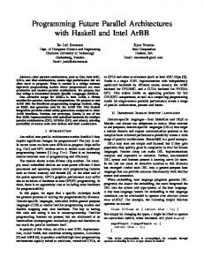
2.1 The PRAM Model In this dissertation the parallel model is the PRAM (see Figure 1). As stated in Chapter 1, PRAM is an acronym that stands for Parallel Random Access Machine. The PRAM is motivated in Chapter 1. A PRAM has an unbounded shared common memory and polynomially many processors indexed from 1 to p(n), where p(n) is a polynomial in the size of the input n. Each processor has its own local memory, and each processor has the same instruction set as the single processor in the RAM model (Aho et al., 1974; Papadimitriou, 1994). All processors run the same program and each processor has access to its own index 8

De nitions and Foundations Processor 1

9 Processor p(n)

Processor 2

Common Memory

Figure 1: A PRAM with p(n) Processors so any processor can execute dierent instructions based on its index. The PRAM model allows a polynomial number of processors to vary with the input size because:

A polynomial number of polynomial time bounded processors can be simulated in polynomial time using one processor.

The power of processors is increasing while their expense and size is decreas-

ing. Therefore, designing algorithms expecting a large numbers of available processors is not unreasonable.

The common memory shared by all of the processors forces us to consider simultaneous memory con icts. The most common distinctions between memory con ict are, exclusive reads (ER) versus concurrent reads (CR), and exclusive writes (EW) versus concurrent writes (CW). Therefore, the CRCW PRAM allows simultaneous reads and simultaneous writes, where the EREW PRAM does not allow simultaneous reads or simultaneous writes. It's easy to imagine several processors simultaneously reading from the same memory location, but to allow simultaneous writes we must decide either which processor \wins" or how to combine the dierent values being simultaneously written. Here are several well-known models of simultaneous write contention:

De nitions and Foundations

10

Priority-CW PRAM: In this model each processor has some given priority, so

memory contentions are resolved by letting the highest priority contesting processor win.

Max-CW PRAM: In this model the processor that is attempting to write the maximum value in the contended memory location wins.

Common-CW PRAM: In this model all processors must write the same value into the contended memory location.

All of the above models can simulate each other within minor time and space factors (Karp and Ramachandran, 1990). Because these parallel models are so closely related, we use the most convenient model at hand.

2.2 Ecient and Optimal Parallel Algorithms The set P is the class of problems that have polynomial time bounded algorithms on a RAM. These problems are often thought to be tractable on modern computers (Garey and Johnson, 1979). Since a PRAM can only have a polynomial number of processors, a RAM can simulate a PRAM in polynomial time. This means the only problems that have any hope of being tractable on a PRAM are those that are tractable on a RAM. Therefore, we will examine the problems in P very closely.

2.2.1 Asymptotic Notation Given an algorithm let In denote the set of all valid inputs of size n. The time complexity of an algorithm A is a function TA from the set of all its inputs to the natural numbers, such that for all i 2 In the value TA(i) is the number of steps algorithm A uses in computing an answer given input i. We write t(n) to denote


11

max f TA (i) g and call this the worst case time complexity for inputs of size n. Time i2In complexity re ects the amount of time it takes an algorithm to solve an instance of a problem. The space complexity of an algorithm is de ned analogously to its time complexity. Space complexity re ects the amount of space it takes an algorithm to solve an instance of a problem. Space complexity includes the space used for all data structures during a computation, but it does not include the space used for the input or the output. We write s(n) to denote the worst case space complexity for inputs of size n. The processor complexity of a parallel algorithm is de ned analogously to space and time complexities. Processor complexity re ects the number of processors it takes a parallel algorithm to solve an instance of a problem. We write p(n) to denote the worst case processor complexity for inputs of size n. In this dissertation the processor, time, and space complexities are always polynomially bounded. The worst case time complexity of a parallel algorithm is the worst case time it takes all processors to nish. The worst case parallel time complexity is also written t(n) for inputs of size n. The following de nitions comprise asymptotic notation. Here all functions are from the positive integers onto the positive integers and all constants are positive. Given two functions f and g, we write f = O(g), if there are two constants c and d such that f (n) cg(n) for all n d. We write f = (g), if there are two constants c and d such that f (n) cg(n) for all n d. We write f = (g) when both f = O(g) and g = O(f ). Call a function f polylog i f (n) = (lgk n) for some constant k > 0. A function f is at most polylog i f (n) = O(lgk n) for some constant k > 0, etc. We will always 1

1

See, for example (Marcus, 1978), for a de nition of a function.


12

attempt to build parallel algorithms that work in polylog time. Further, all polylog and polynomial functions are in terms of the input size n. We write f (n) = O~ (g(n)) i f (n) = O(g(n) lgk n) for some constant k 0. The ~ g(n)) and f (n) = ~ (g(n)) have the expected meanings. expressions f (n) = ( The function f is within a polynomial of g i f (n) = O(gk(n)) for some constant k 1.

2.2.2 Optimality and Work Given a problem , an algorithm is optimal i there is no algorithm that can solve with fewer operations. Likewise, given a problem , an algorithm is asymptotically optimal i there is no algorithm that can solve with asymptotically fewer operations. A problem has time or space complexity f if there is no known algorithm that can solve in better than f time or space, respectively. For a given problem, a parallel algorithm's performance is often compared with the performance of a sequential algorithm that solves the same problem. The most common measure of performance of a parallel algorithm is the algorithm's processortime product. This is the product of the processor complexity and the time complexity of a parallel algorithm. The processor-time product is sometimes called the work of a parallel algorithm. Comparing the work of a parallel algorithm with the work of a sequential algorithm is often done to within a polylog factor to make up for dierences between the models. If the processor-time product of a parallel algorithm is signi cantly less than the time complexity of a sequential algorithm for the same problem, then simulating the parallel algorithm sequentially gives a new and more ecient sequential solution. An ecient parallel algorithm runs in polylogarithmic time and has processortime product within a polylog factor of the best known sequential solution. We allow the processor-time product to be within a polylog time factor of the best sequential


13

solution because dierent variations of the PRAM model are equivalent to within log-time factors. Suppose a problem has an asymptotically optimal sequential solution that costs f , then a polylog time parallel algorithm is asymptotically optimal, if its processor-time product is O(f ). There are other notions of optimality for parallel algorithms. A parallel algorithm has optimal speed if reducing its parallel time complexity forces its processor-time product to increase.

2.3 The Parallel Computation Hypothesis A few technical details are omitted in the following statement of the parallel computation hypothesis since they are not germane to our discussion. Assuming all time and space complexities are at least asymptotically logarithmic, the parallel computation hypothesis is: A parallel model of computation is \reasonable" if the time complexity of a problem on this model is within a polynomial of the space complexity of the same problem on a (sequential) Turing machine, assuming the total work of the parallel and sequential solutions are within a polynomial of each other. Figure 2: The Parallel Computation Hypothesis This is a hypothesis since it assumes that a Turing machine is a \reasonable" sequential model. That is, this hypothesis de nes a \reasonable" parallel model in terms of a \reasonable" sequential model. The Turing machine model is polynomially equivalent to the RAM model, (Aho et al., 1974; Papadimitriou, 1994). Making a few assumptions about the processor word-sizes gives the next theorem (Parberry, 1987), The time complexity of a problem on a PRAM is polynomially equivalent to the space complexity of the same problem on a RAM.


14

As before, this assumes the amount of work on the PRAM is within a polynomial of the work on the RAM. For many dierent parallel models, including variations of the PRAM model, the parallel computation hypothesis is a theorem assuming the RAM model is a \reasonable sequential model." In other words, given a polynomial number of processors a PRAM is a reasonable parallel model. A decision problem is a problem that has only two possible solutions True or False. Decision problems free us from details such as the cost of writing the output. The class NC contains all decision problems solvable in polylog time on a PRAM with a polynomial number of processors. A problem is inherently parallel if it is in NC . An algorithm is NC if it runs in polylog time on a PRAM using a polynomial number of processors. It is unknown whether any problem in P requires polynomial space, although it seems likely that some do. Suppose some problems in P require polynomial space to run. Then by the parallel computation hypothesis these problems cannot run in polylog time using a polynomial number of processors. This is the basis of the theory behind inherently sequential problems. If some problem has polynomial space complexity and there is a log-space transformation from to , then is at least as hard as in terms of the space it uses. (All log-space algorithms run in polynomial time, see (Papadimitriou, 1994).) This is because any instance of can be solved by transforming it, in log-space, to an instance of , and then by solving this instance of we have solved the initial instance of . Therefore, if has log-space complexity, then must also have log-space complexity. On the other hand, say all problems in P can be log-space transformed to , then if any problem in P requires polynomial space, then also requires polynomial space. Alternatively, if can be solved in polylog space, then all problems in P can be too. Of course, if a problem in P takes polynomial space 1

1

2

2

1

1

2

1

2

2

1

2

2

2


15

to solve on a RAM, then by the parallel computation hypothesis it takes polynomial time to solve on a PRAM (with a polynomial number of processors). Next is a sketch of how to show a problem is inherently sequential. Given two decision problems and , the notation / means is reducible to . Saying is reducible to means that: 1

2

1

1

2

1

2

2

1. There is an algorithm that transforms any instance of to an instance of . And for any input to , say i 2 In, then (i) is an input to of polynomial size in n. 1

2

1

2

2. If A solves and B solves then A(i) i B((i)), since and are decision problems the programs A and B can only output either True or False. 1

2

1

2

The notation /t means the reduction algorithm / is polynomially time bounded. In this case, /t is a polynomial-time reduction. Similarly, the notation /s means the reduction algorithm / is logarithmically space bounded. The class P -Complete contains all decision problems in P that appear to require polynomial space on a RAM and are log-space reducible to each other. A problem 2 P is log-space complete for P (P -Complete) i for each 2 P there is a log-space bounded reduction /s such that /s . Generally, a problem is shown to be P -Complete by rst showing that it is in P , then by giving a logspace transformation from some other P -Complete problem to . In terms of parallel computation, this log-space transformation can be replaced by an NC algorithm as a consequence of the parallel computation hypothesis. The rst log-space complete problem in P was given in (Cook, 1974). Such problems are in some sense among the \hardest" in P in that solving them takes as much space as does solving any other problem in P . By the parallel computation hypothesis, a problem in P that appears to take polynomial space on a RAM also appears to take a polynomial amount of parallel 1

1

2

2

'' &' &&


P NC

P -Complete

$$ % $ %%

16

Figure 3: A Hypothetical View of P

time on a PRAM. It seems that only if we augment a PRAM to have an exponential number of processors, then we can solve P -Complete problems on it in polylog time. See Figure 3 for a hypothetical relationship of P -Complete and NC . For ease of exposition, we simply say a problem is NC or P -Complete when it is in NC or it is in P -Complete respectively. If any problem is both NC and P -Complete then NC = P -Complete = P . A problem inherently sequential if it, or its restriction to a decision problem, is P -Complete.

2.4 The Nature of Some Paradigms Not all algorithm design paradigms give ecient parallel algorithms. Standard sequential algorithm design tools, such as depth rst search, and variations of the greedy method, do not seem to give ecient parallel algorithms. The greedy principle applies when every optimal subsolution is in some optimal solution, but there is no method speci ed for getting from the optimal subsolution to a total solution. On the other hand, the lexicographical greedy principle applies


17

when every optimal subsolution is in some optimal solution and this subsolution is built lexicographically into a solution. Here depth rst search to refers to the problem of labeling a graph's nodes in the order they are traversed by some depth rst search. The problem of lexicographical depth rst search is inherently sequential, though the general problem of depth rst search is not known to be either inherently sequential or inherently parallel (Reif, 1985). In (Anderson and Mayr, 1987; Anderson and Mayr, 1987a) it is shown that many problems that have elementary solutions by the lexicographical greedy principle are inherently sequential. This makes many problems that are solvable sequentially using lexicographical reachability intractable to solve in polylog time. Non-lexicographical greedyness is not necessarily bogged down in the same way. On the other hand, since (Valiant et al., 1983), many problems amenable to dynamic programming were known to be NC , but their processor complexities were very high (asymptotically ninth degree polynomials). More recent results have lowered this processor complexity. This dissertation shows that some of these problems have ecient parallel solutions.

2.5 Historical Notes The PRAM model was rst given in (Fortune and Wyllie, 1978). One of the rst renditions of the parallel computation hypothesis was in (Chandra et al., 1981) in terms of alternating Turing machines. Here the main focus was P Space and the polynomial hierarchy to describe a notion of parallelism for Turing machines. This work inspired much work showing the asymptotic equivalence of parallel time and sequential space on the Turing machine model.


18

The authors of (Balcazar et al., 1988 and 1990) say that the conference paper (Chandra and Stockmeyer, 1976) is where the parallel computation hypothesis was rst explicitly mentioned by name. In the same conference (Kozen, 1976) gave a similar rendition of a parallel Turing machine model. Together, both (Chandra and Stockmeyer, 1976) and (Kozen, 1976) lead to the journal article (Chandra et al., 1981). The authors of (Karp and Ramachandran, 1990) point out that the parallel computation hypothesis is quite robust in that most theoretical parallel models of computation abide by it such as those from circuit complexity, parallel vector machines, alternating Turing machines, etc. The class NC stands for \Nick's Class" in honor of Nick Pippenger. The rst P -Complete problem was given in (Cook, 1974) while the author was discussing the question of the space complexity of parsing context-free grammars relative to the space complexity of all problems in P .

Chapter 3 Sequential Dynamic Programming This chapter contains sequential dynamic programming algorithms for the matrix chain ordering problem and an optimal convex polygon triangulation problem. More details about these and other related problems and their sequential solutions can be found in several standard textbooks such as (Aho et al., 1974; Baase, 1988; Cormen et al., 1990; Purdom and Brown, 1985). A dynamic programming problem is a problem that is amenable to a simple and ecient sequential dynamic programming solution.

3.1 The Basics The dynamic programming paradigm is based on the principle of optimality. This principle is that for a structure to be optimal all of its well-formed substructures must also be optimal. Hence, the dynamic programming paradigm is essentially a top down design method. Conversely, the greedy principle basically is that if a substructure is optimal, then it is in some optimal superstructure. In some sense this is a bottom up design method. Some foundations for the principle of optimality and the greedy principle can be 19

Sequential Dynamic Programming

20

found in (Bellman, 1957) and (Cormen et al., 1990; Korte et al., 1991), respectively.

3.2 The Matrix Chain Ordering Problem This section contains an in-depth discussion of the matrix chain ordering problem (MCOP). Its focus is on the classical sequential solution. An optimal convex polygon triangulation problem is also given and is cast in an almost identical framework. A solution of the MCOP can be expressed as a parenthesization of the n given matrices giving an order to optimally multiply them. There are a Catalan number of ways to parenthesize any n element associative product, which is (4n=n = ), hence an exhaustive search algorithm is not feasible. Let denote matrix multiplication and take a chain of n matrices M M Mn, then there are n(n , 1)=2 possible subproducts of the form Mi;j = Mi Mj . Clearly, the nal product M ;n must be made up of one of these subproducts. These subproducts, in turn, are made up of such subproducts with the single matrix base case when i = j . Taking the de nition of Mi;j and applying the principle of optimality gives a dynamic programming algorithm with a polynomial time solution. This was observed by several researchers in the early 1970s. In 1973, the rst polynomial time solutions of the MCOP were given independently in (Godbole, 1973) and in (Muraoka and Kuck, 1973). Godbole's algorithm has become the classical O(n ) dynamic programming solution, and it is where we begin. Start by letting M [i; j ] be the minimal cost of multiplying matrices i through j , therefore our nal goal is to compute M [1; n]. Also M [i; i] is the cost of multiplying 3 2

1

1

2

1

3

The basic matrix multiplication algorithm can be found in almost any standard algorithms textbook, take for example those listed in the beginning of this chapter. 1

Sequential Dynamic Programming

21

matrix i through i, thus M [i; i] = 0. For simplicity, let didj dk be the cost of multiplying two matrices of dimensions di dj and dj dk . The cost of multiplying these two matrices is written f (i; j; k) = didj dk . Generalizations of this matrix product function re ecting asymptotically better matrix multiplication algorithms, such as those in (Pan, 1984; Coppersmith and Winograd, 1990), are also acceptable, see (Chandra, 1975). Given that the matrix Mi;j is of dimensions di dj , and taking M [i; i] = 0 as a base case suggests the following recurrence for solving the MCOP: +1

+1

+1

+1

+1

+1

+1

+1

M [i; k] = imin f M [i; j ] + M [j + 1; k] + didj dk g j :1 otherwise +1

+1

Given ai and aj assume that both ai aj and pc(ai; aj ) can be computed in constant time. That is, for any values of i; j; and k the cost f (i; j; k) can be computed in constant time.

4.2 Greedy Minimum Cost Parenthesizations This section contains a subproblem of the MPP called the greedy parenthesization problem (GPP). We use this problem to develop the MPP and to discuss some previous results.

S ;n Si;i Si;j 1

+1

is the start symbol ! ij i i + 1 = j and i + 1 n ! i (Si ;j ) j (Si;j, ) j i i < j , 1 +1

1

Figure 8: The Grammar L

1

Any string derived from L is a greedy parenthesization of n elements. We consider this to be greedy since this grammar describes an associative product that characterizes \local product growth." Given a weighted semigroupoid, the greedy parenthesization problem (GPP) is to nd minimal products that are generated by the grammar in Figure 8. For every weighted semigroupoid with a greedy associative product of n elements 1

A Dynamic Graph Model

32

we can construct a corresponding weighted digraph. Finding a shortest path in such a graph solves the GPP for the given associative product. Denote vertices by (i; j ), where 1 i j n, and edges by !, " or %. Edge (i; j ) " (i , 1; j ) represents the product ai, (ai aj ), therefore it weighs f (i , 1; i , 1; j ). Similarly, (i; j ) ! (i; j +1) represents the product (ai aj ) aj and it weighs f (i; j; j + 1). Also, for all i; 1 i n, the arrows % represent edges from (0; 0) to (i; i). 1

+1

De nition Given an n-element weighted semigroupoid, the graph Gn = (V; E ) has vertices,

V = f(i; j ) : 1 i j ng [ f(0; 0)g and unit edges,

E = f(i; j ) ! (i; j + 1) : 1 i j < ng [ f(i; j ) " (i , 1; j ) : 1 < i j ng [ f(0; 0) % (i; i) : 1 i ng and a weight function W where

W ((i; j ) ! (i; j + 1)) = f (i; j; j + 1) 1ij s+1 so f (k; s; t) > W ((k; s) ! (k; s+1)). Intuitively, we are trading the associative product cost f (k; s; t) for the rst edge of (k; s) ! ! (k; t). This rst unit edge is cheaper than the associative product cost. +1

+2

With this, because (k; s +1) ! ! (k; t) costs wk kws : wt k and the path (s + 1; s + 1) ! ! (s + 1; t) costs ws kws : wt k and since wk < ws the theorem holds. +2

+1

+2

+1

+1

+1

Otherwise, say there is a horizontal jumper in r to (s + 1; t). Apply this case again inductively, until there is a jumper that derives its weight from a straight unit path. We are trading each jumper's associative product cost for the cost of the rst unit edge in the associated unit path. These rst unit edges are always cheaper than the related associative product cost. Eventually, the shortest path to (k; t) is shown to be (k; k) ! ! (k; t). Hence, r is a unit path, but this means that it must be the straight unit path in row i by Case i. Handling a path with more than one jumper is straightforward. Inductively applying these two cases to jumpers successively farther away from (0; 0) completes the proof. 2 This theorem also holds for a monotone list of weights having the relation

wi > wi > > wj +1

+1

where the shortest path is (0; 0) % (j; j ) " (j , 1; j ) " " (i; j ): Therefore, if the list of weights wi; wi ; : : : ; wj is monotone, then we do not have +1

+1

Special Dn Graphs for the MCOP

59

to construct any jumpers in D(i; j ). We say that D(i; t) intersects D(j; v) i V [D(i; t)] \ V [D(j; v)] ,f(0; 0)g 6= ;. From here on, references to monotone subgraphs assume that the monotone subgraphs do not intersect any canonical subgraphs. This is because canonical subgraphs contain monotone subgraphs, but such monotone subgraphs are not of particular interest to us.

Theorem 11 If D(i; t) does not intersect any canonical graphs and has no critical nodes, then the weight list wi ; wi+1 ; : : : ; wt+1 is monotonic.

Proof: Say there are no critical nodes in D(i; t). Then there is at most one weight wj where j + 1 = 6 1 such that +1

wi > wj > wj < wj < < wt ; +1

+2

+1

otherwise D(i; t) would contain critical nodes. But in this case, since w = min fwig in it must be that D(1; j + 1) contains the critical node (1; j ), which means that D(i; t) would intersect with a canonical subgraph. On the other hand, this means both the row and column equations begin and remain indeterminate so the next fact holds. 1

1

For all (j; j + 2) 2 V [D(i; t)], either wj < wj < wj < wj or wj > wj > wj > wj . Fact 1:

+1

+1

+2

+2

+1

+3

+3

Applying the row or column equations to the nodes (j; j + 2), for all j; i < j t, establishes this fact. For instance, let

R = (wj , wj )kwj : wj k + (wj , wj )wj wj ; +1

+2

+3

+2

+3

then R is order determinant so it must be either wj < wj wj > wj and wj > wj , but not both. +1

+2

+3

+1

+1

and wj

+2

< wj , or +3


60

Suppose wj < wj and wj < wj , and assume that wj > wj , otherwise if wj < wj , then wj < wj < wj < wj so we are done. This means wj < wj and wj > wj , therefore wj > maxfwj ; wj g and this indicates (j; j + 1) is a critical node. This is a contradiction, hence it must be that wj < wj < wj < wj . Using Fact 1, the theorem follows inductively. 2 A lack of critical nodes implies the existence of a monotone subgraph. Just the same, a lack of ANSV matches in a section of a weight list indicates a monotone sublist. Assuming that D(i; t) does not intersect with any canonical graphs gives the next corollary. +1

+1

+2

+1

+2

+3

+1

+2

+2

+1

+2

+3

+1

+1

+2

+1

+2

+3

Corollary 2 If D(i; t) contains no critical nodes, then there are no jumpers in a shortest

path from (0; 0) to (i; t). Moreover, if D(i; t) contains no critical nodes, then the shortest path from (0; 0) to (i; t) is a straight unit path.

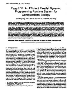
A proof of this follows immediately from Theorems 10 and 11. Take a canonical subgraph D ;m , where all critical nodes have been found and form a unit edge-connected path p. Removing the nodes and adjacent edges of p splits D ;m in two. These two pieces of D ;m are U for upper and L for lower. See Figure 18. (1

(1

)

)

(1

)

(1,n)

w1

U wi

L wj wn+1

Figure 18: A Dn Graph Split by a Path of Critical Nodes, Arrows Point Toward Smaller Weights

Let D(1; s) be the maximal well-formed subgraph of U and let D(s + 1; m) be the


61

maximal well-formed subgraph of L. By the maximality of D(i; t) in U we mean that for any other well-formed subgraph D(j; k), if D(j; k) U then D(j; k) D(i; t).

Theorem 12 (Modality Theorem) If D(1; s) U and D(s + 1; n) L, where both D(1; s) and D(s + 1; m) are maximal, then w < w < < ws and ws > ws > > wm > wm . 1

+3

2

+1

+2

+1

into U and L where D(1; s) and D(s +1; n) are maximal, so (s; s + 1) is a critical node. Therefore, it must be that ws > maxfws; ws g, so ws < ws and ws > ws . By Theorem 11, the weight lists w ; w ; : : : ; ws; ws and ws ; ws ; : : : ; wm; wm are both monotonic. Thus ws < ws , so it must be that w < w < < ws < ws . In addition, because ws > ws , so ws > ws > > wm > wm . 2 i;t canonical graph, then both Take a D j;k

Proof: The path p splits D

(1

;m)

+1

+1

+1

+2

1

2

+1

+1

+1

( (

+2

+2

+1

1

+1

+2

2

+1

+1

+2

+1

) )

wi < wi < < wj and wk > wk > > wt +1

+1

+1

follow from Theorem 12.

5.4 Historical Notes Theorem 5 was rst proved by (Deimel and Lampe, 1979) and a simpler proof was later given by (Hu and Shing, 1982). There seems to be two general approaches to improving the complexity of nding minimal paths in special graphs. The rst is to use speci c properties of the graphs to get more ecient renditions of the (min; +)-matrix based shortest-path algorithms. This approach can be seen in (Aggarwal et al., 1987; Aggarwal and Park, 1988; Apostolico et al., 1990), where they use Monge and monotone properties to improve the processor complexity of the standard (min; +)-matrix multiplication. The second


62

approach breaks the graph up while only keeping a very small fraction of the pieces. These pieces can be worked on in parallel and the results of each of these computations can be joined giving a complete solution to the original problem. The work in this dissertation is based on a divide-and-conquer approach.

Chapter 6 Approximating the MCOP This chapter contains a fast parallel approximation algorithm for the MCOP. This algorithm can run in O(lg n) time using only n=lg n processors on both a commonCRCW PRAM and a EREW PRAM. Alternatively it can run in O(lg lg n) time using n=lg lg n processors on a common-CRCW PRAM. The algorithm given in this section is based on two applications of the ANSV problem.

6.1 A Parallel Approximation Algorithm for the MCOP This section contains a O(lg lg n) time and n=lg lg n processor approximation algorithm for the MCOP. This algorithm is built by combining results of (Chin, 1979), and (Hu and Shing, 1981) with those of (Berkman et al., 1989). This algorithm approximates the MCOP to within 15:5% of optimality. In addition, the processor-time product of this algorithm is linear. This algorithm is not much more than several applications of the ANSV problem, 63

Approximating the MCOP

64

so various processor complexities and times result in applications of Theorem 7. The approximation algorithm consists of two stages. The rst stage isolates relatively heavy weights by nding matrix products that must be in an optimal parenthesization. The isolation of such heavy weights provides optimal substructures that are in optimal superstructures|essentially giving a converse to the principle of optimality. The second stage is simply a greedy approach for nding a parenthesization once we have applied the rst stage of the algorithm. Therefore, this is basically a greedy algorithm, but there are no lexicographical constraints on it. By Corollary 1 rotate any given weight list so that w is the smallest weight. For the next theorem let wi; wi ; and wi be three adjacent weights in a weight list of an instance of the MCOP where wi < wi and wi > wi which together means that wi > maxfwi; wi g. 1

+1

+2

+1

+1

+1

+2

+2

Theorem 13 (Hu and Shing, 1981) If w wiwi + wiwi wi < w wiwi + w wi wi 1

+2

+1

+2

1

+1

1

+1

+2

(3)

then the product (ai ai+1 ) is in an optimal parenthesization.

Proof of this Theorem is left to the literature, see (Chin, 1979) and (Hu and Shing, 1981) for dierent proofs. When wi > maxfwi; wi g fails to hold Equation 3 cannot hold, so there is no gain in assuming wi > maxfwi; wi g. +1

+2

+1

+2

Corollary 3 If Equation 3 holds, then wi > maxfwi; wi g. +1

+2

A proof follows from Equation 3 with

w = min fwig; in 1

and

1

+1

w wi(wi , wi ) + wi wi (wi , w ) < 0 1

+2

+1

+1

+2

1


65

so it must be that wi , wi reassociating gives +2

+1

< 0. Also, starting with Equation 3 again and

w wi (wi , wi ) + wiwi (wi , w ) < 0 1

+2

+1

+2

+2

1

so wi , wi < 0. Unfortunately, the converse of this last corollary is not true. An ANSV match may not represent a minimal parenthesization in the MCOP. But any product that is in a minimal parenthesization by way of Equation 3 has been isolated by some match. Therefore, using the ANSV problem, the values in the weight list approximate the optimal level of parentheses. A list of weights is reduced i for all weights, say wi , with ANSV match [wi; wi ] Equation 3 fails to hold (Chin, 1979). A reduced weight list may be non-monotonic. Generalizing Equation 3 is done as follows. Suppose by Theorem 13 that (ai ai ) is in an optimal parenthesization. Applying Theorem 13 to the list +1

+1

+2

+1

l = w ; : : : wi, ; wi; wi ; wi ; : : : ; wn 1

1

+2

+3

+1

works in the same way. That is, if wi > maxfwi, ; wi g and w wi, wi +wi, wiwi < w wi, wi + w wiwi , then the parenthesization given by the solution of the ANSV problem on l indicates that (ai, ai ) is optimal. Given the weight list l = w ; w ; : : : ; wn the approximation algorithm is (Chin, 1979; Hu, 1982; Hu and Shing, 1981): 1

1

1

1

+2

1

1

+2

1

+2

+2

1

1

+1

2

+1

1. Reduce the weight list l giving the weight list l , renumbering l to be l = w ; w ; : : : ; wr where w = min fwig. ir 2

1

2

+1

1

1

2

2

+1

2. If l has more than two weights, then compute the depths of the parentheses for the linear product (( (a a ) ) ar ) of cost w kw : wr k. With this, 2

1

2

1

2

+1


66

make the parenthesis discovered in Step 1 the appropriate amount deeper. The depth of the parentheses determines the order to multiply the matrices. Next techniques are given to run this algorithm eciently in parallel. Intuitively, by Theorem 13, if the match [wi, ; wi ] represents the nesting level of two parentheses in an optimal product, then we have characterized wi's in uence. Remove wi from the weight list and recursively apply Theorem 13. Suppose in solving the ANSV problem the weight wj has the match [wi; wk ]. Then, if 1

+1

w wiwk + wiwj wk < w wj wk + w wiwj 1

1

1

(4)

and products (ai aj, ) and (aj ak, ) are both in an optimal parenthesization, then the product (ai aj, ) (aj ak, ) is also in an optimal parenthesization. Certainly, by Theorem 13 this is true when i = j , 1 and j = k , 1. In addition, Corollary 3 generalizes to suit Equation 4. A weight list can be reduced by two applications of the ANSV problem as follows. Given the weight list l the next algorithm outputs a reduced weight list. Let A[1 : : : n + 1] be an array of n + 1 integers all initialized to zero. 1

1

1

1

1. Solve the ANSV problem on the weight list l. Next check to see if there are any weights satisfying the condition described by Equation 3. If there are none, then output l since it is reduced, then stop. 2. For all weights wj in l that have matches, say [wi; wk ], if wj and wi; wk ; satisfy Equation 4, then assign a 1 to A[j ]. 3. Now solve the ANSV problem on A[1 : : : n + 1]. If the nearest smaller values of A[j ] are in the match [A[i]; A[k]], then (ai ak, ) is in an optimal parenthesization. Removing all of the weights isolated by optimal parenthesizations 1


67

gives a reduced weight list, which is output. This algorithm produces a reduced weight list and optimal parenthesizations that have been isolated by the conditions of Equation 3. The rst step of this algorithm is correct by Theorem 13 and Corollary 3. The next theorem establishes the correctness of the last two steps of the algorithm.

Theorem 14 If the ANSV match of A[j ] is [A[i]; A[k]] where i < k, then the product (ai ak, ) is in an optimal parenthesization. 1

Proof: The array A contains values from the set f0; 1g, so if A[j ] = 0 then A[j ] does

not have an ANSV match. On the other hand, if A[j ] = 1 then A[j ] must have an ANSV match since A[1] = 0 and A[n + 1] = 0. Now consider the case where A[j ] has match [A[i]; A[k]]. This means for all t such that i < t < k, A[t] also has match [A[i]; A[k]]. All of these matches are compatible, consequently all A[t] = 1 for i < t < k are nested ANSV matches. This means there must be at least one list of three consecutive weights, say wt; wt ; and wt , that satisfy Equation 3. Now remove the middle such weight, wt , and recursively continue this argument knowing that Equation 4 has marked the other such weights. 2 By Theorem 7, the three steps of this algorithm cost O(lg lg n) time using n=lg lg n processors on the common-CRCW PRAM or in O(lg n) time using n=lg n processors on a EREW PRAM or a common-CRCW PRAM. Assume that r +1 weights remain after reduction. Then renumbering and rotating the list of remaining weights gives w ; w ; ; wr where w = min fwig. The ir second step of the approximation algorithm requires that we form the appropriate linear product with the remaining matrices. The depth of the parentheses provides an approximation to within 15:5% of optimal for the MCOP. This is due to (Chandra, 1975), (Chin, 1979), and (Hu and Shing, 1981). +1

+1

1

2

+1

1

1

+1

+2


68

Theorem 15 (Hu and Shing, 1981) If a weight list w ; w ; ; wr is reduced, 1

2

+1

then the MCOP can be solved to within a multiplicative factor of 1:155 from optimal in constant time using n processors. This is done by choosing the linear parenthesization (( (a1 a2 ) ) ar,1 ) ar .

That is, after a weight list is reduced choosing a linear parenthesization with cost w kw : wr k gives a matrix chain product that is within a multiplicative factor of 1:155 from optimal. The approximation algorithm given here is another problem whose solution is built on the ANSV problem. This algorithm also shows that only a linear number of entries of a dynamic programming table give a nice approximate solution to the MCOP. That is, a minor variation of the path of critical nodes in the canonical subgraphs supply a good approximate solution for the matrix chain ordering problem. This algorithm is built on the greedy principle more than the dynamic programming paradigm. In terms of the processor-time product, this algorithm is optimal. 1

2

+1

6.2 Historical Notes Both (Chandra, 1975) and (Chin, 1979) gave approximations for the MCOP that were not quite as good as the 1:155 of Theorem 15. Theorem 15 was conjectured in (Chin, 1979) and nally proved in (Hu and Shing, 1981). The algorithm given in this chapter appeared in (Bradford, 1992; Bradford, 1992a) and a very similar algorithm was given in (Czumaj, 1992). The content of this chapter is almost identical to that which the author of this dissertation submitted to the Symposium on Parallel Algorithms and Architectures (SPAA) 1992.

Chapter 7 An O~(n3)-Work Polylog-Time Algorithm This chapter contains an O(lg n)-time algorithm for solving the matrix chain ordering problem that uses n =lg n processors. Throughout this chapter leaf subgraphs of the form D i;j are written as D ;m where 1 m n. In addition, assume that Dn contains critical nodes, otherwise by Corollary 2 there is an immediate exact solution. One of the key insights of this chapter is that canonical subgraphs can be treated atomically while nding a shortest path in a Dn graph. Further, (min; +)-matrix multiplication joins these subgraphs together to form a shortest path in an entire Dn graph. 3

3

(

)

(1

)

7.1 Shortest Paths Without Critical Nodes This section culminates with Theorem 18 which basically states that in a D ;m graph shortest paths have a very rigid structure; this result supplies the rst step for nding shortest paths in canonical subgraphs. All results in this section apply to shortest paths from (0; 0) to (1; m) in D ;m (leaf) graphs and to shortest paths from (j; k) to (1

(1

)

69

)

An O~ (n )-Work Polylog-Time Algorithm

70

3

i;v (band) graphs. (i; v) in D j;k A path q with one jumper contains no critical nodes i there are no critical nodes in q and there are no critical nodes in q's dual path. That is, a jumper (i; j ) =) (i; k) contains no critical nodes if both (i; j ) and (i; k) are not critical nodes and there are no critical nodes in a shortest path contributing to this jumper's weight. This generalizes to paths with more than one jumper. In our terminology the following result of (Hu and Shing, 1982, Corollary 3) can be stated as: ( (

) )

Theorem 16 In any canonical graph, the sum of the two products wiwj wk + +1

+1

wj wj wk where i < j < k, cannot contribute to the weight of any shortest path i w k > wj > w i . +1

+1

+2

+1

+1

Next is a useful technical lemma.

Lemma 6 In a D

(1

;m)

graph if (i; t) 2 V [U ], then wi < wt+1 .

Proof: Since (i; t) 2 V [U ] and i < t, there must be some critical node (i; u) 2 V [p] where t < u. This means that wj > maxfwi; wu g, for all j; i < j u. Since i < t < u it must be that wi < wt . 2 A symmetric argument to that of Lemma 6 shows that wi > wj for all nodes (i; j ) 2 V [L]. +1

+1

+1

Theorem 17 Any shortest path q to some vertex (i; j ) in D critical nodes, except possibly (i; j ), is a straight unit path.

(1

;m)

where q contains no

A proof of this theorem follows from an inductive application of Lemma 4 and Theorem 12. The last theorem and all previous results of this section also apply to shortest i;v canonical subgraphs. paths from (j; k) to (i; v) in D j;k ( (

) )


71

3

Jumpers of the form (i; j ) =) (i; k) such that (j +1; k) 2 V [p] are very important. Such jumpers contain at least one critical node, namely (j + 1; k).

Lemma 7 If a horizontal shortest path q to (i; u) 2 V [U ] [ V [p], is such that q has one jumper (i; j ) =) (i; k) and (j + 1; k) 2 V [p], then q is equivalent to a shortest path to (j + 1; k) followed by (j + 1; k) * (i; k) ! ! (i; u). The same holds for any such vertical path. A proof of this lemma follows from Lemma 1 and Theorem 2. That is, this lemma is based on the Duality Theorem. Suppose (j; k) and (i; t) are two critical nodes in a canonical graph D ;m , where i j k t. Then there is a unit path of critical nodes from (j; k) to (i; t). With this, there are two important symmetric paths between (j; k) and (i; t): The upper angular path of (j; k) and (i; t) is (1

)

(j; k) * (i; k) ! ! (i; t) and the lower angular path of (j; k) and (i; t) is (j; k) =) (j; t) " " (i; t) A trivial angular path has only two unit edges and no jumpers. That is, if the three unit edge connected critical nodes (j; k) ! (j; k + 1) " (j , 1; k + 1) then there is a trivial angular path (j; k) " (j , 1; k) ! (j , 1; k , 1) where (j , 1; k) is not a critical node. For examples of angular paths see Figure 19.


72

3

In a canonical subgraph the shortest path between any two critical nodes that contains no other critical nodes is an angular path. Angular paths are central to the rest of this dissertation. (i,t)

(j,k)

Figure 19: Two Angular Paths A central result of this section is that a shortest path to a critical node (i; j ) in a canonical graph may be along a path of critical nodes, then through an angular path then back to a subpath of critical nodes, then through an angular path and back to a subpath of critical nodes, etc. In our terminology, Hu and Shing gave the following important theorem.

Theorem 18 (Hu and Shing, 1982) A shortest path to a critical node (i; j ) in a

D

graph is either along a straight unit path to (i; j ), along the path of critical nodes to (i; j ), or along subpaths of critical nodes connected together by angular paths and nally to (i; j ). (1

;m)

A proof of this theorem follows inductively from Theorem 17 and the following. Say that there is some jumper (i; j ) =) (i; k) such that (j + 1; k) 62 V [p]. Then, since W ((i; j ) =) (i; k)) = f (i; j; k) + sp(j + 1; k) and assume without loss that (j + 1; k) 2 V [L], see Figure 20a. Now, by Theorem 17 we know the shortest path to (j + 1; k) includes the unit edge (j + 2; k) " (j + 1; k) which has cost wj wj wk . Additionally, assume that (j +2; k) 62 V [p]. But, because f (i; j; k) = wiwj wk and since (i; j ) and (i; k) are in U Lemma 6 indicates that wi < wj < wk . Therefore +1

+1

+1

+1

+1

+1


73

3

applying Theorem 16 shows that the jumper (i; j ) =) (i; k) can't be in a minimal path in Dn. A similar case holds for Figure 20b. (i,j)

(i,k)

(i,j)

(j+1,k)

(i,k) (j+1,k)

(j+1,j+1)

(k,k)

(a)

(b)

Figure 20: Two Jumpers and their Complimentary Paths By the Duality Theorem and the compatibility of critical nodes, any jumpers over p have dual paths containing no jumpers over p giving the last case just discussed. (i,j)

(i,k)

(i,j)

(i,k)

Figure 21: Two Jumpers Over the Path p This last theorem and the next corollary also hold for shortest paths from (j; k) i;v graphs. to (i; v) in D j;k ( (

) )

Corollary 4 A shortest path from (0; 0) to a non-critical node (s; t) in a D

;m)

graph is either a straight unit path, or it is a minimal path to some critical node (i; j ) and from (i; j ) to (s; t) by an angular path. (1


74

3

7.2 Combining the Canonical Graphs This section gives a parallel divide and conquer tool for nding minimal paths in Dn graphs based on work of Hu and Shing. This is done by isolating an underlying tree structure connecting the canonical subgraphs, so we can nd shortest paths in these subgraphs individually while essentially ignoring the eect of the monotone subgraphs. This allows the computation of a shortest path in a Dn graph by applying variations of tree contraction techniques. These techniques incorporate special \leaf pruning" operations. As before, by Corollary 1 rotate any given weight list so that w is the smallest weight. Next we present, without proof, a central result of Hu and Shing. In essence, this result gives some of the power of the greedy principle together with the principle of optimality. That is, this result allows the isolation of some substructures that are necessarily in an optimal superstructure. 1

Theorem 19 (Hu and Shing, 1982) Given a weight list w ; : : : ; wn with the three 1

+1

smallest weights w1 < wi+1 < wv+1 and i + 1 < v , the products w1 wi+1 and w1 wv+1 are in some associative product(s) in an optimal parenthesization.

There may be one or two f s that contain the products w wi and w wv . The next corollary is central to the results of this section. It essentially guarantees that certain easily computable nodes are a part of a shortest path in a given Dn graph. Where Hu and Shing use the results of the last theorem as a sequential divide and conquer tool, here it is made into a parallel tool. 1

+1

1

+1

Corollary 5 (Atomicity Corollary) Given a weight list w ; : : : ; wn with the three 1

+1

smallest weights w1 < wi+1 < wv+1 and i + 1 < v , the critical nodes (1; i) and (1; v ) are in a shortest path from (0; 0) to (1; n) in Dn .


75

3

A proof follows directly from Theorem 19. Suppose w < wi < wv are the three smallest weights in Dn and both D ;i and D i ;v are leaf subgraphs. Then there is a shortest path from (0; 0) to (1; i) in D ;i . Applying Corollary 5 to the subgraph D(1; v), which also has the three smallest weights w < wi < wv , shows that (1; i) is in a minimal path to (1; v). Therefore by the structure of Dn graphs the only contribution that D i ;v can make to a shortest path to (1; v) is by providing sp values for jumpers along the unit path (1; i) ! ! (1; v). That is, there may be some jumper (1; j ) =) (1; k) such that (j + 1; k) 2 V [D i ;v ] and 1

( +1

+1

(1 )

+1

)

(1 )

1

+1

+1

( +1

( +1

)

)

(1; i) ! ! (1; j ) =) (1; k) ! ! (i; v) is cheaper than

(1; i) ! ! (1; v):

Shortly, in Lemma 9, we will see that we only have to consider jumpers (1; j ) =) (1; k) such that (j + 1; k) is a critical node in D i ;v . ( +1

)

7.2.1 Canonical Trees Dividing a Dn graph into a tree of canonical subgraphs using Corollary 5 is easily done in O(lg n) time with n=lg n processors by solving the ANSV problem. In a Dn graph the structure joining all of the critical nodes is a canonical tree, see also Hu and Shing (Hu and Shing, 1980; Hu and Shing, 1982; Hu and Shing, 1984). De ne the leaves, edges, and internal nodes of a canonical tree as follows. Initially, in every canonical subgraph D ;m the critical node (1; m) is a leaf and is denoted by (1; m) to distinguish it from other critical nodes. A D ;m canonical subgraph only contains one tree node, namely (1; m). All other tree nodes will also be overlined. An isolated critical node is a critical node with no critical nodes that are one unit (1

)

(1

)


76

3

edge away. The internal tree nodes are isolated critical nodes or (i; v) and (j; k) for i;v canonical graphs, where k 6= j + 1. A D i;v graph only contains the two tree D j;k j;k nodes (i; v) and (j; k). Notice that all tree nodes are also critical nodes, thus they are compatible. The edges of a canonical tree are the straight unit paths that connect tree nodes. Jumpers may reduce the cost of tree edges. An edge from (i; j ) to (i; k) is denoted by (i; j ) ! ! (i; k) and all edges are directed towards (1; n). Since tree nodes are critical nodes with easily discernible properties, they are eciently distinguishable in parallel. In addition, we can discard all monotone subgraphs since they have no in uence on a shortest path to (1; n), except if D(1; j ) is monotone and w = min fw g. That is, since w = min fwig, if D(1; i) is monotone for some ij i in i, then a shortest path to (1; n) will travel along the path (1; 1) ! ! (1; i). But this is the only case when a monotone graph contains a piece of a minimal path from (0; 0) to (1; n). For the next lemma, assume w = min fwig. in ( (

) )

( (

1

1

1

1

1

1

) )

+1

+1

Lemma 8 In a monotone subgraph D(i; k) of Dn, the cost of a shortest path to (i; k) for i > 1 plus the associative weight f (1; i , 1; k) is more than the unit path (1; i , 1) ! ! (1; k). Proof: Since D(i; k) is monotone, we either have wi < < wk or wi > > wk . So by Theorem 10, the shortest path to (i; k) in D(i; k) is either (i; i) ! ! (i; k) or (k; k) " " (i; k). Therefore, taking the jumper (1; i , 1) =) (1; k) with weight sp(i; k) + f (1; i , 1; k) we have two cases. +1

Case

+1

i: The ordering of the weight list is wi < < wk . +1

In this case, the shortest path to (i; k) is (i; i) ! ! (i; k). Clearly, f (1; i , 1; k) = w wiwk and W ((1; i , 1) ! (1; i)) = w wiwi . But since 1

+1

1

+1


77

3

wi wk , it must be f (1; i , 1; k) W ((1; i , 1) ! (1; i)). Along the same lines, W ((1; j ) ! (1; j + 1)) < W ((i; j ) ! (i; j + 1)) holds for all j; i j < k. +1

Case

+1

ii: The ordering of the weight list is wi > > wk . +1

In this case, the shortest path to (i; k) is (k; k) " " (i; k). Since f (1; i , 1; k) = w wiwk , W ((1; k , 1) ! (1; k)) = w wk wk , and wi wk , it must be that f (1; i , 1; k) W ((1; k , 1) ! (1; k)). Along the same lines, W ((1; i + j , 1) ! (1; i + j )) < W ((i + j + 1; k) " (i + j; k)) for all j; 0 j < k , i. 1

+1

1

+1

2

Suppose Dn has fewer than n , 1 critical nodes. Then Dn may have several disconnected canonical trees and one or more monotone subgraphs by Corollary 2. But, by Theorem 9 there is at least one path from (0; 0) to (1; n) joining these canonical subtrees. From Lemma 8, after discarding irrelevant monotone subgraphs and for the i;v graphs, there are several structures that D ;m graphs may moment ignoring D j;k form together. The relationships of tree nodes is the basis of all of these structures. Let (i; j ); (j + 1; k); : : : ; (u + 1; v) be neighboring leaves in D(i; v) such that they are all in a canonical tree rooted at (i; v) or in no canonical tree at all. All of these leaves together can have the next relationships, or combinations of them. ( (

) )

(1

)

1: The leaves are not joined together by internal tree nodes. For instance, this case occurs if wi < wj < < wu < wv .

Case

+1

+1

+1

2: The leaves form a binary canonical tree, see Figure 22. In this case, there are internal tree nodes in D(i; v) that connect the leaves together.

Case

Solving Case 1 is done by treating it as an instance of Case 2 by building a surrogate tree. The viability of treating these situations as Case 2 is now shown.


78

3

Figure 22: A Canonical Tree of D

(1

;m)

Graphs, the Circles Denote Tree Nodes

Take a list of r monotone leaves, none of which are in a canonical tree. Label the leaves (i; j ); (j + 1; k); (k + 1; t); : : : ; (u + 1; v) and without loss assume that wi < wj < < wu < wv so these leaves are all in D(i; v). Now, by Corollary 5 tree node (i; j ) must be in a shortest path from (0; 0) to (i; v). Therefore, applying the Theorem 2, a shortest path from (0; 0) to (i; v) goes from (0; 0) to (j + 1; v) and then over the tree edge (j + 1; v) " " (i; v). Now, complete this argument by induction. Band subgraphs also form trees in the same way. Trees containing band subgraphs are treated in the same way as above. +1

+1

+1

7.3 Finding Shortest Paths to All Critical Nodes in Canonical Subgraphs i;v This section discusses an algorithm for nding shortest paths in D ;m and D j;k canonical graphs. As before, p denotes the continuous path of critical nodes in a i;v graph. D ;m or D j;k First an m =lg m processor and O(lg m)-time algorithm for nding a shortest path to all critical nodes in a D ;m leaf subgraph is given. This is done by treating angular paths as edges so p is now an (m +1)-node graph with (m ) edges. That is, any angular path (j; k) * (i; k) ! ! (i; t) connecting the critical nodes (j; k) and (i; t) becomes one edge from (j; k) to (i; t) costing W ((j; k) * (i; k))+ wikwk : wt k. (1

(1

)

( (

( (

)

) )

2

3

(1

)

2

+1

+1

) )


79

3

Of course, since (j; k) is a critical node but (i; k) is not a critical node and both are in the same canonical graph, it must be that

W ((j; k) * (i; k)) = wikwi : wj k + f (i; j , 1; k): +1

i;v canonical graphs. Further, using a Now by Theorem 17, this also holds for D j;k (min; +)-matrix multiplication shortest path algorithm, nding shortest paths in such an (m + 1)-node graph costs O(lg m) time with m =lg m processors. This results in a polylog time and n =lg n processor MCOP algorithm at the end of this chapter. Next is the O(lg m) time and m =lg m processor algorithm for nding a shortest path to each critical node in a D ;m graph. First compute all of the unit paths to nodes in p in constant time using m processors. Perhaps, we can best view these paths as edges from (0; 0) to the nodes in p. Further, the cost of each of the (m ) angular paths can be computed in constant time using m processors, with preprocessing costing O(lg m) time and m=lg m processors. The preprocessing is just computing parallel partial pre x minima. Compute the shortest path to each node in p by treating every angular path as a weighted edge and applying a parallel (min; +)-matrix multiplication all pairs shortest path algorithm to the nodes in p. This algorithm costs O(lg m) time and m =lg m processors, and provides a shortest path from (0; 0) to every critical node in a D ;m graph. Compute the shortest paths from (0; 0) to all critical nodes in a i;v canonical graph in the same way. D j;k ( (

2

) )

3

3

2

3

(1

)

2

2

2

3

(1

( (

)

) )

Theorem 20 Given a D

;m)

graph computing a shortest path from (0; 0) to all nodes in p takes O(lg2 m) time using m3 =lg m processors. (1

i;v This theorem also holds for nding shortest paths from all critical nodes in a D j;k canonical graph to (i; v). ( (

) )

An O~ (n )-Work Polylog-Time Algorithm 3

80

7.3.1 Leaf Pruning and Band Merging Here a basic technique for joining band canonical subgraphs quickly in parallel is given. This technique is based on edge minimization and builds shortest paths in Dn graphs. Take the two jumpers (i; j ) =) (i; t) and (i; k) =) (i; u) in row i and without loss say j < k. Then these jumpers are not compatible i k < t < u. If (j +1; t) 2 V [p] and (k + 1; u) 2 V [p], then (j + 1; t) and (k + 1; u) are compatible. Consequently, any two jumpers in row i such as (i; j ) =) (i; t) and (i; k) =) (i; u), where (j + 1; t) 2 V [p] and (k + 1; u) 2 V [p0], must be compatible, where p and p0 are possibly distinct paths of critical nodes. Notice that if p and p0 are distinct, then they are still compatible. Given a Dn graph with the jumpers (i; j ) =) (i; t) and (i; k) =) (i; u), let p be a minimal path from (0; 0) to (1; n) in Dn. Then all jumpers (i; j ) =) (i; t) and (i; k) =) (i; u) such that (j + 1; t) 2 V [p] and (k + 1; u) 2 V [p] are compatible. Minimizing the cost of a straight unit edge path in a canonical tree by using jumpers is edge minimizing, and we will show that the jumpers only have to get their sp values from critical nodes. Only tree edges or straight unit paths will be edge i;v graphs. For example, let p be the path of critical nodes in D(k; t) minimized in D j;k and consider the straight unit path (i; j ) ! ! (i; v). If the jumper (i; k) =) (i; t) is such that (k + 1; t) 2 V [p] and ( (

) )

(i; j ) ! ! (i; k) =) (i; t) ! ! (i; v) is cheaper than (i; j ) ! ! (i; v), then we edge minimize (i; j ) ! ! (i; v) with (i; k) =) (i; t). The next procedure edge minimizes the unit path along the ith row to the critical


81

3

node (i; v) with all jumpers that get their sp values from the critical nodes V [p],

A[i; v] =

f wikwi : wv k; wikwk : wu k , wikwk : wu k + W ((i; k) =) (i; u)) g min

8(k+1;u)2V [p]

+1

+1

+1

+1

+1

+1

and the same can be done for straight vertical unit paths. The minimal cost along the tree edge i to (i; v) is in A[i; v], assuming only one connected path of critical nodes p. Notice by Theorem 6 that we can compute the cost of the straight unit (sub)paths in constant time with one processor with the appropriate preprocessing.

Lemma 9 When edge minimizing a tree edge (i; j ) ! ! (i; v) in a canonical subgraph we only have to consider jumpers (i; k) =) (i; t) such that (k + 1; t) 2 V [p]. Proof: Take row i, and (i; i) ! ! (i; v) assuming that some jumper (i; s) =) (i; t) minimizes row i where (s + 1; t) 62 V [p] and i < s < t u. Without loss, say (s + 1; t) 2 V [U ], so a shortest path to (s + 1; t) is either the straight unit path (s + 1; s + 1) ! ! (s + 1; t) or this unit path with jumpers by Corollary 4.

All jumpers getting their sp value from a critical node in p must be compatible. Therefore, there is only one jumper that gets its sp value from a critical node in a shortest path from (s + 1; s + 1) to (s + 1; t). Now there are three cases to consider. i: A minimal path to (s + 1; t) is the straight unit path (s + 1; s + 1) ! ! (s + 1; t).

Case

By the Duality Theorem the minimal path along (i; i) ! ! (i; s) =) (i; t) is equivalent to the path (s + 1; s + 1) ! ! (s + 1; t) * (i; t):


But

(s + 1; s + 1) ! ! (s + 1; t) * (i; t)

is not an angular path, a straight unit path, or a path of critical nodes intermixed with angular paths getting their sp value from p. Therefore, we arrive at a contradiction of Corollary 4. ii: A shortest path to (s + 1; t) is along the unit path from (s + 1; s + 1) to (s + 1; t) and contains one or more jumpers whose sp values are not from V [p].

Case

This case would imply that a shortest path from (0; 0) to nodes in U are not angular paths or straight line unit paths contradicting Corollary 4. iii: A shortest path to (s +1; t) is along the unit path from (s +1; s +1) to (s + 1; t) and contains one jumper that gets its sp value from a critical node in p.

Case

Let (s + 1; j ) =) (s + 1; k) be a jumper such that (j + 1; k) 2 V [p]. Thus by the Duality Theorem the path (s + 1; s + 1) ! ! (s + 1; j ) =) (s + 1; k) ! ! (s + 1; t) followed by the jumper (s + 1; t) * (i; t) costs the same as the path (i; i) ! ! (i; s) =) (i; t): At the same time, the path (s + 1; s + 1) ! ! (s + 1; j ) =) (s + 1; k) ! ! (s + 1; t)

82


83

3

is equivalent to a shortest path to (j + 1; k) followed by the angular path (j + 1; k) * (s + 1; k) ! ! (s + 1; t), by the Duality Theorem. This means a shortest path from (0; 0) to (i; t) is from (0; 0) to (j + 1; k) then (j + 1; k) * (s + 1; k) ! ! (s + 1; t) * (s + 1; t); but this is a contradiction by Corollary 4, since this path is not an angular path. Cases i and ii can occur at the same time, though the above arguments still hold. 2 This lemma easily generalizes to the case where p is a path of critical nodes in a conglomerate of canonical subgraphs. Lemma 9 also highlights the role well-formed subsolutions play in the dynamic programming solution of the MCOP. Let p be a minimal path from (0; 0) to (k; t) in D(k; t). Then Lemma 9 extends to the case of only jumpers (i; k) =) (i; t) along tree edges (i; j ) ! ! (i; v) such that (k + 1; t) 2 V [p].

Theorem 21 When edge minimizing a tree edge (i; j ) ! ! (i; v) in a canonical subgraph we only have to consider jumpers (i; k) =) (i; t) such that (k + 1; t) 2 V [p]. Proof: Since (i; j ) ! ! (i; v) is a tree edge it must be that maxfwi; wv g < ws for all s; i s v + 1. For the sake of a contradiction suppose the jumper (i; k) =) (i; t), such that (k + 1; t) 62 V [p] but (k + 1; t) 2 V [p], is the jumper that minimizes the tree edge (i; j ) ! ! (i; v) more than any other jumper. But since (k + 1; t) 62 V [p], it's safe to assume that the angular path +1

(r; s) * (q; s) ! ! (q; u)


84

is the angular path in p that goes around (k + 1; t), so (r; s) 2 V [p] and (q; u) 2 V [p]. In this case, by Theorem 2 a minimal path to (q; u) is (q; q) ! ! (q; r , 1) =) (q; s) ! ! (q; u) such that (r; s) 2 V [p]. In particular, notice that the jumper (q; k) =) (q; t) saves no more than any other jumper by edge minimizing the unit path (q; q) ! ! (q; u) and, since (i; j ) ! ! (i; v) is a tree edge, we know that wi < wq and f (i; k; t) < f (q; k; t). Thus, if (q; k) =) (q; t) saves no more than the jumper (q; r , 1) =) (q; s) in row q, then (i; k) =) (i; t) saves no more than any other jumper in row i. 2 This last theorem is very important. It says once a minimal path p is discovered in a subgraph D(j; k), then during edge minimization we only have to consider jumpers with sp values from p. Of course V [p] V [p], where p is the path of critical nodes.

Theorem 22 Given a tree node (i; u) where the graph D(i; u) contains the leaves D(i; j )

and D(j + 1; u) so (i; j ) and (j + 1; u) are tree nodes, if D(j + 1; u) is a canonical subgraph, then a shortest path from (i; j ) to (i; u) can be found in O(u , j ) operations.

Proof: Since (i; j ); (i; u); and (j +1; u) are all critical nodes, the three smallest weights

in wi; : : : ; wu are wi; wj ; and wu . Now assume without loss that wi < wu < wj . Hence, by Corollary 5, tree node (i; j ) must be in a shortest path from (0; 0) to (i; u). Therefore, edge minimize the unit path (i; j ) ! ! (i; u). Otherwise, if wu < wi < wj then (j + 1; u) is in a shortest path from (0; 0) to (i; u). Therefore by the Duality Theorem we can edge minimize the path (i; j ) ! ! (i; u). There could be a quadratic number of jumpers of the form (i; k) =) (i; t) such that j k < t u. But by Theorem 21 we only have to consider jumpers along row i that get their sp values from p. That is, only jumpers such as (i; k) =) (i; t) where (k + 1; t) 2 V [p]. The appropriate value of sp, which has been computed for each node in p, can be retrieved and added to the appropriate value of f in constant +1

+1

+1

+1

+1

+1

+1


85

3

time. Therefore nding the minimal values for the paths between nodes (i; j ) and (i; u) takes O(u , j ) operations, since there are O(u , j ) such compatible jumpers. 2 The O(u , j ) operations are easily done in O(lg(u , j )) time using (u , j )= lg(u , j ) processors. In O(lg(u , j )) time and with (u , j )= lg(u , j ) processors rst get all of the jumper values and then nd the minimal such jumper. The last theorem holds for leaves in the canonical tree that have been combined and become conglomerates of other leaves and internal nodes. In this situation, jumpers derived from critical nodes in dierent subtrees are independent and compatible, so we can minimize tree edges with them simultaneously. But, canonical i;v must be considered. In this case, take the leaf D(j; k) subgraphs of the form D j;k i;v , where D(j; k) consists of the pruned subgraphs D(j; t) that must be pruned in D j;k and D(t + 1; k). If there is a shortest path through (j; k) to (i; v), then by Corollary 5 and depending on whether wj < wk or wk < wj either (j; t) or (t + 1; k), respectively, are in shortest paths to (j; k). Therefore, by Theorem 22 we would be done. But we must address the possibility that the cost of paths from (0; 0) to critical nodes throughout D(j; k) can contribute to shortest paths to critical nodes from (j; k) to (i; v). In fact, we must combine the information about shortest paths in D(j; k) with information i;v . The combining of this shortest path information is about shortest paths in D j;k i;v with sp values from critical nodes of done by edge minimizing unit paths in D j;k D(j; k). The next theorem is another parallel divide and conquer tool, but it is for merging i;v graph. a D(j; k) leaf into a D j;k ( (

) )

( (

) )

+1

+1

( (

) )

( (

( (

) )

) )

i;v graph with a shortest path p from (j; k) to (i; v ) and suppose Theorem 23 In a D j;k ( (

) )

the four smallest weights are wi < wv+1 < wi+1 < wv , then p goes through one of 1. Either (i + 1; v ) or (i + 1; v , 1) or both


86

3

2. (i; i + 1) and (i; v , 1) 3. (v , 1; v ) and (i + 1; v ) i;v graph, it must be that Proof: Since wi < wv < wi < wv and we are in a D j;k (i; v); (i + 1; v); and (i + 1; v , 1) are all critical nodes, so p may go through them. Clearly, if p goes through (i +1; v , 1), then p cannot go through (i; i +1) or (v , 1; v). +1

( (

+1

) )

If the shortest path p has a jumper up to row i, then (i; i + 1) will be in p in the sense of Theorem 9. Of course, if p goes through (i; i + 1), then p cannot go through either (v , 1; v) or (i + 1; v). Finally, if (v , 1; v) is in a shortest path to (i; v), then (i + 1; v) is also and both (i; i + 1) and (i + 1; v , 1) are not in this minimal path. 2 This theorem also holds for D ;m graphs. By Theorem 23 take a shortest path from (0; 0) to (i; v) that goes through (i; i +1). Then there might be a straight unit path (i; i + 1) ! ! (i; v) connecting (i; i + 1) and (i; v). On the other hand, there may be some jumper (i; j ) =) (i; k) such that (1

)

(i; i + 1) ! ! (i; j ) =) (i; k) ! ! (i; v) is cheaper than (i; i + 1) ! ! (i; v). The only possible ways to merge canonical graphs together are in Figure 23. Merging the two leaf canonical graphs as in Figure 23a is leaf pruning, and Figures 23b,c are band merging. Leaf pruning can be accomplished by edge minimizing after all shortest paths to critical nodes in the leaves have been found. In Figure 23c, contracted trees A and B are used to edge minimize the unit paths marked by \Min-A" and \Min-B." Edge minimizing the unit paths in the outer band with the contracted trees gives an instance of Figure 23b. i;v with D j;t takes O(lg m) time using m = lg m processors, assuming Merging D j;t k;s ( (

) )

( (

) )

2

3


87

3

Min−B

A

B

Min−B

c)

b)

a)

Min−A

Min−A

Figure 23: The Variations of Band Merging or Leaf Pruning i;v has a total of m critical nodes. Let p be a minimal path from (i; v ) back to D k;s i;v , and let p be a minimal path from (j; t) back to (0; 0) only (0; 0) only through D j;t j;t . Now, merging these two graphs by nding all the angular paths from through D k;s i;v . Next, applying an all pairs critical nodes in p forward to any critical nodes in D j;t shortest path algorithm combines these bands giving a shortest path from (i; v) back i;v . to (0; 0) through D k;s ( (

) )

1

( (

( (

) )

2

) )

( (

2

( (

) )

) )

7.3.2 Contracting a Canonical Tree This subsection shows how to use edge minimization and band merging as the prune operations for a standard tree contraction algorithm. Together these algorithms complete a good algorithm for the MCOP. This algorithm has work O~ (n ) and runs in polylog time. In a tree that contains only D ;m canonical subgraphs, each prune operation is an edge minimization that joins leaves together, until the entire canonical tree is one leaf. Every critical node (i; j ) has an associated variable sp(i; j ) where sp(i; j ) denotes the cost of a shortest path from (0; 0) to (i; j ). Further, a canonical tree has at most n , 1 critical nodes, so only O(n) such variables are necessary. Initially, all internal tree nodes have sp(i; j ) = 1 and all nodes in p which are tree leaves have the minimum value from (0; 0) to (i; j ) stored in sp(i; j ). That is, in i;v the tree leaves the minimal paths p have been computed. In addition, for all D j;k 3

(1

)

( (

) )


88

3

graphs compute and store the value of the shortest path from all critical nodes in i;v to (i; v ). Compute these initial values using the methods of Subsection 7.3. D j;k Also, each tree edge (i; j ) ! ! (i; k) initially has weight wikwj : wk k. After the appropriate preprocessing, by Theorem 6, computing the initial cost of each of these O(n) tree edges costs constant time with one processor. Assume the standard tree contraction algorithm (JaJa, 1992; Karp and Ramachandran, 1990; Kumar et al., 1994) except for the prune operation. Along with the new prune operation, there is an ordering of the leaves that prevents the simultaneous pruning of two adjacent leaves. Take two neighboring canonical graphs D i;j and D j ;k with the two leaves (i; j ) and (j + 1; k) and the internal node (i; k), say wi < wk < wj . Then prune leaf (j + 1; k) since (i; j ) is in a shortest path from (0; 0) to (i; k) by Corollary 5. Otherwise, say wk < wi < wj , then prune leaf (i; j ). While, standard tree contraction algorithms use the Euler tour technique (JaJa, 1992; Karp and Ramachandran, 1990) to number the leaves appropriately, as just seen the canonical nodes often provide a natural prune ordering. The viability of this natural leaf numbering follows by induction. Thus apply the Euler tour technique in case the leaf ordering is arbitrary, otherwise take the natural pruning order. Take the tree made by connecting the two leaves (i; j ); (j + 1; k) to the internal node (i; k), then the pruning order is arbitrary if wi = wj = wk . Also, the numbering of tree nodes by the Euler tour technique prevents a band graph from being merged simultaneously with both the band inside it and the band around it. See standard tree contraction techniques for details of this use of the Euler tour technique. Figure 24 depicts a canonical tree rooted at (i; k) that is the parent of tree nodes (i; j ) and (j + 1; k) which are siblings representing D(i; j ) and D(j + 1; k), respectively. Assume that D(j + 1; k) has been pruned into a leaf, and if wk < wi < wj , then compute what contribution, if any, (j + 1; k) makes to the shortest path to (i; k). ( (

) )

+1

+1

(

( +1

)

)

+1

+1

+1

+1

+1

+1

+1

+1


89

3

[i,j]

[i,k]

[i,u]

[j+1,k]

Figure 24: A Small Canonical Tree

Figure 25: A Linear List of Tree Leaves This is determined by edge minimizing the tree edge (i; j ) ! ! (i; k) with all nodes in a minimal path from (0; 0) to (j + 1; k). After this edge minimization, inactivate (j + 1; k) and its parent (i; k), so (j + 1; k) will not be pruned again. The tree leaves depicted in Figure 25 can be pruned in any order. They are \pruned into" the edge joining them by rst nding minimal paths to all critical nodes in each leaf. And then edge minimizing the edge joining them all with jumpers that get their sp values from the critical nodes in the leaves. A linear list of leaves as those in Figure 25 can be pruned in any order. Therefore, choosing to do them simultaneously makes most sense. But, any number of nested bands must be merged in a way to avoid con icts. This is easily done using the Euler tour technique for numbering appropriately for tree contraction, see (Karp and Ramachandran, 1990). The next lemma shows that pruning allows the construction of a shortest path from (0; 0) to (1; n) in a tree made of leaf canonical graphs and isolated critical nodes. This is necessary for canonical subtrees as in Figure 22. Let Dn0 only contain leaf subgraphs and isolated tree nodes.


90

3

Lemma 10 Tree contraction of a tree of D

;m)

graphs with isolated internal tree nodes correctly computes a shortest path from (0; 0) to (1; n) in Dn0 . (1

Proof: The proof is by induction on the tree node depth, where a leaf is of depth 1.

The case where the depth d = 1 is trivial, so consider when the depth is d = 2. Without loss say the canonical tree of depth 2 has nodes (i; j ); (j + 1; k); and (i; k), (see the subgraph D(i; k) in Figure 24). Now by Corollary 5 and since wi; wj ; and wk are the three smallest weights in the list wi; : : : ; wk it must be that (i; j ) or (j + 1; k) is in a shortest path from (0; 0) to (i; k). Thus, the prune operation above processes this properly. Suppose the prune operation is correct for all trees Td of depth d, and take the tree Td of depth d + 1. Without loss, say Td contains two subtrees of depth d and the root of Td is (i; k). In addition, if the two depth d subtrees of Td have roots (i; j ) and (j + 1; k), then by the properties of critical nodes, we know that the three smallest weights in wi; : : : ; wk are wi; wj ; and wk . Without loss, say wk < wi < wj , which by Corollary 5 tree node (i; j ) must be in a shortest path from (0; 0) to (i; k). By the inductive hypothesis, if all the subtrees rooted at (i; j ) and (j + 1; k) have been pruned, then there is a shortest path from (0; 0) to (i; j ) and another to (j + 1; k). Pruning leaf (j + 1; k) nds all critical nodes that are in each of the two subtrees rooted at (i; j ) and (j + 1; k). The pruning operation is just an edge minimization to see which combinations of critical nodes may from a shortest path form (0; 0) to (i; k). 2 The tree pruning of Lemma 10 takes O(lg n) time using n=lg n processors following standard tree contraction techniques. Either Corollary 5 gives the leaf pruning ordering, or they can be pruned arbitrarily where we would choose an ordering like the one given by the Euler tour technique. +1

+1

+1

+1

+1

+1

+1

+1

+1

+1

+1

2

+1


91

3

i;v and D k;t , where j k < t Lemma 11 Given two nested canonical graphs D j;u r;s ( (

) )

( (

) )

u, with no such canonical subgraph between them, we can join them with one merge operation.

A proof of this follows the proof of Lemma 10 in a straightforward manner. Assume that the shortest paths in all canonical subgraphs are computed rst at a cost of O(lg n) time and n =lg n processors. Independently, compute the shortest paths of all of these canonical subgraphs. Then the pruning algorithm takes O(lg n) time using n =lg n processors. Now considering Lemmas 11 and 10 we can solve the MCOP by performing tree contraction with the prune operation. Analyzing this algorithm gives the following theorem. 2

3

2

3

Theorem 24 We can solve the MCOP in O(lg n) time using n =lg n processors. 3

3

This algorithm uses O(n) nodes in a Dn graph to solve the MCOP. Thus we can solve the MCOP by using only O(n) elements of a classical dynamic programming table. Theorem 24 also applies to the optimal convex triangulation problem with the standard triangle cost metrics (Cormen et al., 1990; Hu and Shing, 1982).

7.4 Historical Notes The algorithm outlined here is basically from (Bradford, 1992). An extended abstract was published in (Bradford, 1992a) and the full version is in (Bradford, 1992b). The full version was available and circulated since May of 1992. Other parallel algorithms for the MCOP with better work were also reported in: (Czumaj, 1993; Ramanan, 1992; Ramanan, 1993; Bradford et al., 1992).


92

The model used in this chapter is important for the study of ecient parallel algorithms for the MCOP and other problems. Furthermore, it is nice to have a re-characterization of Hu and Shing's work on the MCOP.

Chapter 8 An O(lg2 n) Time and n Processor Algorithm This chapter contains an O(lg n) time algorithm for solving the matrix chain ordering problem that uses n processors on either the common-CRCW PRAM or an EREW PRAM. This algorithm can be adapted to take O(lg n) time and use n=lg n processors on either of these models. The best algorithms in this chapter have processor-time products of O(n lg n) just a lg n factor from the work of the sequential algorithm of Hu and Shing. Further, our algorithms will have processor-time products of O(n lg n) if an algorithm is discovered that has takes O(lg n) time and n=lg n processors for nding the row minima of totally monotone matrices. This chapter starts by isolating the n =lg n processor bottlenecks of the O(lg n) time and O~ (n ) work algorithm from the last chapter. The rst key insight of this chapter is that a carefully constructed inductive invariant allows the replacement of the brute force all-pairs shortest paths algorithm by successive applications of parallel partial pre x and binary search algorithms. This blasts the process complexity from n =lg n down to n=lg n or n=lg lg n, or even n depending on the desired time complexity. The algorithms with these processor complexities have O(n lg n) total work. 2

3

2

2

3

3

3

3

93

An O(lg n) Time and n Processor Algorithm

94

2

The next central insight is that both the time and work can be improved by using ecient parallel algorithms for computing row minima of totally monotone matrices.

8.1 The n3=lg n Processor Bottlenecks This section gives the n =lg n processor bottlenecks of the main algorithm in Chapter 7. Three parts of the algorithm in Chapter 7 use n =lg n processors. All other parts of this algorithm use a total of n=lg n processors and take O(lg n) time. The three bottlenecks are: Finding shortest paths from all critical nodes in leaf graphs back to (0; 0), see Figure 26a. Merging two bands, see Figure 26b, and merging two bands that have contracted canonical trees between them, see Figure 26c. In Figure 26c, contracted trees A and B are used to edge minimize the unit paths marked by \Min-A" and \Min-B." Edge minimizing the unit paths in the outer band with the contracted trees gives an instance of the second bottleneck, see Figure 26b. Edge minimizing the unit paths in the outer band with the contracted trees costs O(lg n) time with n =lg n processors. Section 8.5 shows how to perform such edge minimization in O(lg n) time with n=lg n processors. Finding shortest paths back to (0; 0) from all critical nodes in a leaf graph, as in Figure 26a, is done by breaking it into nested bands. Therefore, nding ecient parallel methods of band merging and edge minimization gives an ecient parallel algorithm for the MCOP. So, nding ecient ways to get shortest paths from all critical nodes back to (0; 0) by edge minimization in leaf subgraphs partitioned as bands is the focus of the rest of this chapter. i;v , let p i;v denote a shortest path from (i; v ) back to (0; 0) Given the band D j;t j;t i;v totally contained in D j;t , see Figure 27. When there is no ambiguity, p i;v j;t will be written as p. 3

3

2

2

( (

( (

) )

) )

( (

) )

( (

) )


95

2

Min−B

A

c)

b)

B

Min−B

a)

Min−A

Min−A

Figure 26: Bottlenecks 1, 2, and 3 for the n =lg n Processor Algorithm 3

i;v , whenever p = p i;v starts from the front critical node of the Given a band D j;t j;t band, then the nodes V [p] are super-critical nodes. Take the minimal path back from the front critical node in Figure 27, only the two black critical nodes are super-critical nodes. Super-critical nodes of a band are all of the critical nodes in some minimal path from the front critical node back to (0; 0). Any two super-critical nodes in p are connected by super-critical nodes interspersed with angular paths by Theorem 18. When a canonical tree of Dn is totally contracted then the nal path p from (1; n) back to (0; 0) gives the optimal order to multiply the set of n matrices. In addition, the cost of p is the minimal cost of multiplying the given chain of n matrices. ( (

) )

( (

) )

8.2 A Metric for Minimal Cost Angular Paths This section gives a metric for nding a minimal cost angular paths by using the equivalence of angular paths and jumpers along unit paths. This equivalence comes directly from Theorem 2. When merging two bands, a unit path has at most one jumper minimizing it since all of the relevant jumpers are nested. These jumpers get their sp values from super-critical nodes of the inner band. The in uence of an angular edge can be taken as a jumper in a straight unit path

An O(lg n) Time and n Processor Algorithm 2

96

(0,0)

Figure 27: The Dashed Path IS p and the Two Black Nodes Are Super-Critical Nodes by Theorem 2. In the case of Figure 26c, any unit edge minimization using sp values from A or B is independent of unit edge minimization using sp values from the inner band. Therefore, measuring the potential contribution of angular edges to straight unit shortest paths is done by measuring the potential contribution of jumpers to shortest paths along straight unit paths. Take a node (s; t) 2 V [p], where sp(s; t) is the cost of a shortest path back to (0; 0), with respect to a band, then in row i we want to compare the cost of the jumper (i; s , 1) =) (i; t) with the cost of the associated unit path (i; s , 1) ! ! (i; t). Given (s; t) 2 V [p], take row i above p with the jumper (i; s , 1) =) (i; t), de ne i (s; t) = wikws : wt k , [ sp(s; t) + f (i; s , 1; t) ]: +1

If i (s; t) > 0, then the jumper (i; s , 1) =) (i; t) provides a cheaper path along row i than the unit path (i; s , 1) ! ! (i; t). In particular, take both (s; t) 2 V [p] and


97

2

(x; y) 2 V [p], and the two possible jumper nestings of Figure 28. a)

(i,s−1)

(i,x−1)

(i,y)

(i,t)

(i,x−1)

(i,s−1)

(i,t)

(i,y)

b)

Figure 28: Two Dierent Nestings of Two Jumpers For the nesting of jumpers of Figure 28a, if i (s; t) > i(x; y) > 0, then the jumper (i; s , 1) =) (i; t) \saves more" than the jumper (i; x , 1) =) (i; y) along row i because (i; s , 1) =) (i; t) doesn't have to deal with the paths (i; s , 1) ! ! (i; x , 1) and (i; y) ! ! (i; t) as well as i (s; t) > i(x; y) > 0. Similarly, for the nesting of Figure 28b, if i(x; y) > i (s; t) > 0, then the jumper (i; x , 1) =) (i; y) \saves more" than the jumper (i; s , 1) =) (i; t) along row i. Notice, in nesting of Figure 28b, if i(s; t) > i(x; y) > 0, then the jumper (i; s , 1) =) (i; t) may or may not make row i cheaper than the jumper (i; x , 1) =) (i; y). But on the other hand, for Figure 28b, if (i; s , 1) =) (i; t) makes row i cheaper than the jumper (i; x , 1) =) (i; y) does, then i(s; t) > i (x; y) > 0. In D ;m , if (s; t) 2 V [p], then above the path of critical nodes p, the function i(s; t) is de ned for all rows i such that s > i 1. Edge minimizing a unit paths is only half of the game, since we must also consider the shortest paths forward. Figure 29 is for the next theorem, see also (Hu and Shing, 1982). (1

)

i;v and any two critical nodes (j; u) and (k; t) in Theorem 25 Given a leaf graph D r;s ( (

) )

i;v such that there is a unit path from (k; t) to (j; u), then a shortest path from (j; u) D r;s to (i; v ) costs less than a shortest path from (k; t) to (i; v ). ( (

) )


98

2

(i,v)

(j,u) (k,t)

Figure 29: (j; u) Shadowing (k; t)'s Shortest Path Forward A proof follows inductively by shadowing trivial angular paths without any jumpers then showing that any shortest path from (k; t) forward to (i; v) can be shadowed by a shorter path from (j; u) forward to (i; v) then taking into account the f values. See Figure 29. Theorem 25 also holds for shortest paths forward in leaf graphs. The next theorem will also be useful.

Theorem 26 Say (i; s , 1) =) (i; t) is in a shortest path forward, and in the next band merging the value of sp(s; t) decreases due to an edge minimization of row s or a lower row, then (i; s , 1) =) (i; t) is still in a shortest path forward.

A proof of this theorem follows directly from the basic notions of shortest paths. In particular, if the shortest path forward from the critical node (s; t) goes through (s; t) * (i; t), then making the path to (s; t) shorter will not eect the jumper (s; t) * (i; t) or the path from (i; t) to the front node of the present band.


99

2

8.3 A Polylog-Time and n2=lg n Processor MCOP Algorithm This section contains an O(lg n) time and n =lg n processor algorithm for the MCOP. This algorithm works by using a key induction invariant that allows recursive doubling techniques to break through the bottlenecks given in the last section. The basic idea of the algorithm is the following. All critical nodes know their shortest paths to the front of the present bands they are in. Only super-critical nodes have their shortest paths back to (0; 0) thorough their present bands. When merging two bands, by Theorem 21, we only have to consider shortest paths from super-critical nodes in the inner band to any critical node in the outer band. Therefore, all critical nodes must maintain a shortest path to the front of the band they are in. At the same time, all super-critical nodes must maintain a shortest path backwards to (0; 0) through the band they are in. This section supplies the details and correctness of this algorithm. Each critical node in Dn has two pointers called front-ptr and back-ptr that represent angular edges. Back-ptr-s are only used by super-critical nodes. With each front-ptr there are two values, cost-of-front-ptr and cost-to-front; and with each backptr there is one value cost-to-back. Cost-of-front-ptr is the cost of the single angular edge going forward from the present node to the front critical node in the present band. Where, the value of cost-to-front is the cost to the front critical node of the present band containing front-ptr. Similarly, the value of cost-to-back is the cost from the super-critical node at hand back to (0; 0) through the present band. Initially, these pointers connect critical nodes and tree edges in the canonical tree. i;v and D j;t be nested bands with paths of critical nodes labeled p i;v and Let D j;t k;s j;t j;t p k;s , respectively. Note (i; v) and (j; t) are the front critical nodes of these bands. As j;t before, p i;v j;t and p k;s are shortest paths from the front critical nodes back to (0; 0) 2

( (

( (

) )

( (

) )

) )

( (

) )

( (

) )

2

( (

) )


100

2

i;v and D j;t , respectively. Let p i;v and p j;t be made by two through the bands D j;t k;s j;t k;s linked lists of back-ptr-s along super-critical nodes back to (0; 0) in their bands. It turns out that the shortest paths forward from all critical nodes in each of these bands are made up of linked lists of trees of front-ptr-s. We will see that this linked list of trees of front-ptr-s is interconnected through the super-critical nodes as in Figure 31. ( (

) )

( (

) )

( (

) )

( (

) )

1. All critical nodes in both bands have their front-ptr-s in trees of shortest paths that eventually go to super-critical nodes which go to the front critical nodes of their respective bands. 2. In the two bands both shortest paths back to (0; 0) of super-critical nodes are known. These shortest paths of super-critical nodes are made of linked lists of back-ptr-s from the front critical nodes of each band back through their respective bands to (0; 0). Figure 30: An Inductive Invariant for Band Merging Figure 30 gives the induction invariant for merging two bands. Figure 31 gives an example of the data structures for maintaining the inductive invariant. In this gure only critical nodes are shown and the super-critical nodes are black. The solid arrows are front-ptr-s and the dashed arrows are back-ptr-s. Suppose (s; t) is a critical node but not a super-critical node, that is (s; t) 2 V [p] and (s; t) 62 V [p]. There is a unique angular edge (x; y) * (r; y) ! ! (r; u) in p that \goes around" (s; t), see Figure 32. Given a canonical graph and take all rows above p then wi < wr implies that row i is \above" row r as in Figure 32. From here on the focus is on nding shortest paths above the path p of critical nodes, the


101

2

Outer Band

Inner Band

Figure 31: Solid Arrows: Forward Linked Lists of Trees; Dashed Arrows: Backward Linked Lists p symmetric case of shortest paths below the path p of critical nodes follows. i;v are edge minimized with jumpers that get their sp values If all unit paths in D j;k j;k , then we can nd the shortest path from (i; v ) back from super-critical nodes in D s;t i;v . First take one processor at each critical node in D i;v that to (0; 0) through D s;t j;k sums the cost of the path back to (0; 0) possibly through an edge minimized unit path with the cost of its shortest path forward. Next, nd the minimal of all of these j;k . sums, giving the shortest path from (i; v) back to (0; 0) through D s;t The basic intuition for the next lemma is if the shorter of two nested jumpers edge minimizes a unit path r, then any unit path above r with both of these jumpers is not minimized by the longer jumper, see Figure 33. Assume there is a unit path of critical nodes from (x; y) to (s; t) to (r; u) as in Figure 32 for the next lemma. ( (

) )

( (

( (

) )

) )

( (

( (

) )

) )

Lemma 12 Given a critical node (s; t) between the super-critical node (x; y) and critical


102

2

(i,y)

(i,u)

(r,y)

(r,u)

(s,t)

(x,y)

Figure 32: (s; t) 62 V [p] and the Angular Edge (x; y) * (r; y) ! ! (r; u) node (r; u) and say i < r < s < x and row i is above row r, that is wi < wr , where rows i and r are above p then

if r (x; y) r (s; t), then i (x; y) i(s; t) Proof: Start with r (x; y) r (s; t) which gives that, wr kwx : wy k , [ sp(x; y) + f (r; x , 1; y) ] +1

is larger than or equal to

wr kws : wt k , [ sp(s; t) + f (r; s , 1; t) ] +1

and a little algebra gives the following (where kwi : wik = 0),

wr [ kws : wxk + kwy : wt k ] < sp(s; t) , sp(x; y) + wr (wswt , wxwy ) +1

+1

+1

+1

and sp(s; t) , sp(x; y) is always positive because (r; x , 1) =) (r; y) is nested inside of (r; s , 1) =) (r; t) and f (r; s , 1; t) < f (r; x , 1; y). Therefore, if sp(x; y) > sp(s; t), then a shortest path p would go through (s; t) to (r; u) and not over (s; t).


103

2

In particular if sp(x; y) > sp(s; t), then since f (r; x , 1; t) > f (r; s , 1; t), it must be that sp(x; y) + f (r; x , 1; t) > sp(s; t) + f (r; s , 1; t). Therefore row r would have been edge minimized by jumper (r; s , 1) =) (r; t) and not by (r; x , 1) =) (r; y), see Figure 33. Row i s-1

x-1

y

t

Row r y

s-1 x-1

t

Figure 33: Two Jumpers in Dierent Rows In addition, wswt , wxwy < 0 since both (x; y) and (s; t) are critical nodes where s x < y t, so it must be that wxwy , wswt > 0. Therefore, since +1

+1

+1

+1

wr [ kws : wxk + kwy : wt k + wxwy , wswt ] < sp(s; t) , sp(x; y) +1

+1

+1

+1

holds and because wi < wr and the term sp(s; t) , sp(x; y) is independent of i and r then it must be that i(x; y) i (s; t). 2 The next theorem follows from Lemma 12.

Theorem 27 Given a critical node (s; t) between the super-critical node (x; y) and

critical node (r; u) and say i < r < s < x and row i is above row r, that is wi < wr , where rows i and r are above p then

if (r; x , 1) =) (r; y) makes row r cheaper than (r; s , 1) =) (r; t) does, then (i; x , 1) =) (i; y) makes row i cheaper than (i; s , 1) =) (i; t) does. A proof follows from Lemma 12 and by the fact that the rows (i; s , 1) ! ! (i; x , 1) and (i; y) ! ! (i; t)


104

2

are cheaper than (r; s , 1) ! ! (r; x , 1) and (r; y) ! ! (r; t) and the change in f values between (r; x , 1) =) (r; y) and (i; x , 1) =) (i; y) is greater than the change of f values between (r; s , 1) =) (r; t) and (i; s , 1) =) (i; t). That is, f (r; x , 1; y) , f (i; x , 1; y) > f (r; s , 1; t) , f (i; s , 1; t) since wx and wy are both bigger than ws and wt , in addition wr > wi therefore, +1

+1

(wr , wi)[wxwy , wswt ] > 0: +1

+1

Given two nested bands with paths of critical nodes pi for the inner band and po for the outer band. Where, pi and po are shortest paths from the front critical nodes back to (0; 0) in each of these bands. Suppose (s; t) is between (x; y) and (r; u) and (s; t) 2 V [pi] and if (x; y) 2 V [pi] and (r; u) 2 V [po], then Lemma 12 and Theorem 27 also hold. This is because sp(s; t) , sp(x; y) is positive by an argument similar to that in the proof of Lemma 12.

Outer Band

Inner Band

Figure 34: Con icting Angular Paths Between Two Bands Being Merged


105

2

Two angular edges above p, say (x; y) * (r; y) ! ! (r; u) and

(i; j ) * (s; j ) ! ! (s; t);

are compatible if they don't cross each other. Compatibility also holds for angular paths below p. Theorem 28 shows that when merging two bands and computing shortest paths forward, only compatible angular edges need to be considered. Figure 34 shows two con icting angular paths. a;z , D d;v , and D g;t , where D g;t is nested inside Take the canonical graphs D c;x e;u d;v a;z a;z and of D e;u which is, in turn, inside of D c;x , see Figure 35. And assume that D c;x d;v are to be merged together then in the next recursive doubling step the new D e;u a;z will be merged with the leaf D g;t . We can assume D g;t is a leaf or a band D e;u band. ( (

( (

( (

) )

) )

( (

( (

) )

(

)

(

)

) )

( (

) )

( (

) )

(

)

(

(a,v)

(a,z)

)

(a,z)

D(c,x)

(b,u)

(b,y)

(c,x)

(d,v) (d,v)

D (e,u)

(e,u) (g,t) (g,t)

D

a;z , D d;v and the Leaf D g;t Figure 35: The Bands D c;x e;u ( (

) )

( (

) )

(

)

) )


106

2

The next theorem assumes we have found a shortest path from super-critical nodes d;v , through critical nodes in the outer band D a;z , see Figure 35. Of course, in D e;u c;x d;v (d; v) 2 V [p e;u ] and without loss assume ( (

) )

( (

( (

) )

) )

(e; u) * (d; u) ! ! (d; v) is in p d;v e;u . Suppose the angular edge ( (

) )

(e; u) * (b; u) ! ! (b; y) a;z is in p a;z e;u , that is the minimal path from (a; z ) back to (0; 0) through D e;u . ( (

) )

( (

) )

Theorem 28 In merging two nested bands computing shortest paths forward from supercritical nodes of the inner band, we can consider only compatibly nested angular edges.

Proof: Suppose for the sake of a contradiction, (e; u) * (b; u) ! ! (b; y) is in p a;z e;u , that is the angular edge ( (

) )

(e; u) * (b; u) ! ! (b; y) a;z , see Figure 35. Take is in a shortest path from (a; z) back to (0; 0) through D e;u d;v , therefore (d; v ) is between (e; u) and (a; z ) in D a;z . Now, (d; v) in the band D e;u e;u a;z g;t when merging D with D e;u we will show that a shortest path forward to (a; z) that goes through (d; v) must go through a critical node in row b or a critical node in some row below b. ( (

( (

(

)

) )

) )

( (

( (

) )

) )


107

2

a;z with D d;v there is some shortest Now assume otherwise, say after merging D c;x e;u path from (0; 0) through (d; v) to (a; z) traveling through an angular path connecting a;z and D d;v and this angular path is con icting with the angular path the bands D c;x e;u ( (

( (

) )

( (

) )

( (

) )

) )

(e; u) * (b; u) ! ! (b; y): Say, without loss, this con icting angular path is (d; v) * (a; v) ! ! (a; z); see Figure 35. These are con icting angular paths since the shortest path from (d; v) forward goes through an angular path that terminates above row b, and the shortest path forward from (e; u) goes through an angular path that terminates in row b. But, a;z the shortest path from (a; z ) back to (0; 0) still goes through the angular in D e;u edge (e; u) * (b; u) ! ! (b; y): ( (

) )

a;z the angular edge In D e;u ( (

) )

(d; v) * (a; v) ! ! (a; z) can't be the shortest path forward from (d; v). By Theorem 2, the shortest path to (b; y) through the angular edge (e; u) * (b; u) ! ! (b; y) is equivalent to the path (b; b) ! ! (b; e , 1) =) (b; u) ! ! (b; y):


108

And since p a;z e;u goes through ( (

) )

(e; u) * (b; u) ! ! (b; y); the jumper (b; e , 1) =) (b; u) edge minimizes row b. Thus, the jumper (b; d , 1) =) (b; v) saves at most as much as (b; e , 1) =) (b; u) and at the same time (b; d , 1) =) (b; v) is nested around (b; e , 1) =) (b; u) which means b(e; u) b(d; v): Also, by Theorem 2, the shortest path from (d; v) to (a; z) that is through the angular edge (d; v) * (a; v) ! ! (a; z) is equivalent to the path (a; a) ! ! (a; d , 1) =) (a; v) ! ! (a; z) But, consider the path, (a; a) ! ! (a; e , 1) =) (a; u) ! ! (a; z) and it must be that (a; e , 1) =) (a; u) is nested inside of (a; d , 1) =) (a; v). In this case, it is possible that d = e or u = v but not both. Since (d; v) is between (e; u) and (b; y) and a < b and wa < wb where row a is above row b and they both are above p, and since the appropriate values are de ned, the following holds by Lemma 12,

if b (e; u) b(d; v), then a (e; u) a (d; v).


109

2

Therefore, a (e; u) a (d; v) which means the jumper (a; e , 1) =) (a; u) saves at least as much as the jumper (a; d , 1) =) (a; v) in a path to (a; z). And because (b; e , 1) =) (b; u) edge minimizes row b, by Theorem 27 and since a (e; u) a (d; v) the jumper (a; e , 1) =) (a; u) saves more in row a than (a; d , 1) =) (a; v). Now, letting

A = (a; a) ! ! (a; e , 1) =) (a; u) ! ! (a; v) D = (d; d) ! ! (d; e , 1) =) (d; u) ! ! (d; v) * (a; v) see Figure 36. (a,a)

(d,d)

(a,e −1)

(a,u)

(d,e−1)

(d,u)

(a,v)

(a,z)

(d,v)

Figure 36: The Two Paths A and D a;z by Path A is a cheaper than path D going from (a; z) back to (0; 0) in D e;u Theorem 27. Now, if (d; v) * (a; v) is in a shortest path forward from (d; v), then the shortest path forward from (e; u) must be through the angular path ( (

(e; u) * (a; u) ! ! (a; z)

) )


110

2

and not the angular path (e; u) * (b; u) ! ! (b; y) which is a contradiction. This comes from the application of Theorem 27 to the jumpers (b; d , 1) =) (b; v) and (b; e , 1) =) (b; u) in row b and then up to row a, since (b; y) is between (d; v) and (a; z). a;z then none of the angular Now, suppose D g;t is merged with the outer band D e;u a;z change. This paths connecting super-critical nodes in D g;t with paths forward D e;u case is a straightforward application of the proof above and Theorem 26. 2 It is important to note that Theorem 28 only shows that angular paths that all start from super-critical nodes in the same path back to (0; 0) are compatible. Theorem 28 doesn't say that all angular paths are always compatible. Suppose, there is some angular path from a super-critical node in the inner band, say (s; t), to the outer band that is in a shortest path from the front node of the outer band back to (0; 0). Then all super-critical nodes from (s; t) back to (0; 0) have their shortest paths forward through the angular path starting at (s; t). On the other hand, all super-critical nodes after (s; t) up to the front super-critical node of the inner band have their shortest paths through nested angular paths connecting the inner and outer bands by Theorem 28. In fact, we can inductively apply this argument together with Theorem 25 giving: (

( (

)

(

)

) )

( (

) )

Corollary 6 Take the nested angular paths connecting two bands that are shortest paths forward from the dierent super-critical nodes of the inner band, then listing the path containing the outermost such angular path to the path containing the innermost such angular path gives more and more costly paths forward.

The next lemma assumes we are merging two nested bands to nd a shortest path from the front critical node of the outer band back to (0; 0).


111

2

Lemma 13 Given a critical node (s; t) and take the ith and rth rows above p such that i < r < s and wi < wr , then we have i (s; t) < r (s; t).

Proof: The function i (s; t) measures (i; s,1) =) (i; t)'s potential minimizing eect on the path (i; i) ! ! (i; u) where (i; u) 2 V [p] and i < s < t u. The cost of the jumper (i; s , 1) =) (i; t) is sp(s; t) + f (i; s , 1; t). Therefore, the dierence i (s; t) , i (s; t) is, +1

(wi , wi)[ kws : wt k , wswt ] +1

+1

+1

where wi > wi. Since the expression kws : wt k , wswt is independent of the dierence of weights wi and wi and kws : wt k, wswt > 0, because (s; t) 2 V [p], also when s = t , 1 gives +1

+1

+1

+1

+1

+1

kws : wt k = wsws + ws wt : +1

+1

+1

+1

In addition, since (s; t) 2 V [p], it must be that maxfws; wt g < wu, for s < u t, thus maxfws; wt g < ws . Therefore, +1

+1

+1

wsws + ws wt +1

+1

+1

> wswt

+1

and the proof follows inductively. 2 The proof of the next lemma is similar to that of Lemma 12. The basic intuition here is that if the longer of two nested jumpers edge minimizes a unit path r, then any unit path below r, with both of these jumpers, is not minimized by the shorter jumper, see Figure 37. This next lemma only considers super-critical nodes since the focus here is on merging two nested bands. Assume there is a unit path of critical nodes from (v; z) to (x; y) for the next lemma.


112

2

Lemma 14 Given two super-critical nodes (v; z) and (x; y) where r < s < x < v and

wr < ws such that rows s and r are above p, then we have

if r (x; y) r (v; z), then s(x; y) s(v; z) Proof: Start with r (x; y) r (v; z) which can be written out as the next expression,

wr kwx : wy k , [ sp(x; y) + f (r; x , 1; y) ] +1

which is greater than or equal to

wr kwv : wz k , [ sp(v; z) + f (r; v , 1; z) ]: +1

By Lemma 13 and since each of these jumpers is of length at least 2 it must be that wr wv wz < wr kwv : wz k and wr wxwy < wr kwx : wy k. In addition, since wr < ws it must be that f (r; x , 1; y) < f (r; v , 1; z) and wr kwx : wy k > wr kwv : wz k and the same holds in row s, therefore s(x; y) s(v; z). 2 +1

+1

+1

+1

+1

Row r

x−1

v−1

y

z

Row s x−1

v−1

+1

z

y

Figure 37: Two Jumpers in Dierent Rows

Theorem 29 Given two super-critical nodes (v; z) and (x; y) where r < s < x < v and wr < ws such that rows s and r are above p, then we have

if (r; x , 1) =) (r; y) makes row r cheaper than (r; v , 1) =) (r; z) does, then (s; x , 1) =) (s; y) makes row s cheaper than (s; v , 1) =) (s; z) does.


113

2

A proof of this theorem follows from Lemma 14 and the fact that the change of the f values between (r; v , 1) =) (r; z) and (s; v , 1) =) (s; z) increases faster than the change in the f values between (r; x , 1) =) (r; y) and (s; x , 1) =) (s; y). i;v and D j;t to form p i;v the next lemma shows that we only While merging D j;t k;s k;s need shortest path values backwards to (0; 0) from super-critical nodes. That is, we don't need shortest path values backwards to (0; 0) from any other critical nodes. Hence, the back-ptrs will form a linked list between super-critical nodes backwards eventually to (0; 0) and we can compute the cost-to-back weights using a parallel pointer jumping partial pre x. ( (

) )

( (

( (

) )

) )

j;t respectively, for any critical nodes Lemma 15 Take p i;vj;t and p j;tk;s in D j;ti;v and D k;s i;v in the outer band, say (u; z ) 2 V [p i;v j;t ] and (u; z ) 62 V [p k;s ], we don't need shortest ( (

) )

( (

) )

( (

( (

paths back to (0; 0).

) )

( (

) )

) )

( (

) )

j;t and D i;v . Proof: Take the angular path (x; y) * (q; y) ! ! (u; z) between D k;s j;t j;t i;v i;v That is (x; y) 2 V [p k;s ] and (u; z) 2 V [p j;t ] but suppose, (u; z) 62 V [p k;s ]. Notice ( (

( (

) )

( (

) )

that (u; z) may be a super-critical node in p i;v j;t . Take the next cases, ( (

) )

( (

( (

) )

) )

i;v is merged with another band nested around it. Then i: Suppose D k;s since (u; z) is not in V [p i;v k;s ] by Theorem 21 we do not have to consider any angular paths starting from (u; z) going forward to critical nodes in i;v . the band nested around D k;s

Case

( (

) )

( (

) )

( (

Case

) )

i;v is merged with a smaller band inside D(k; s). ii: Suppose D k;s ( (

) )

Node (u; z) could be the terminal node of an incoming angular path contributing to a shortest path forward for some super-critical node in D(k; s). In this case (u; z) needs to have a shortest path from (u; z) forward. Of course, in this case (u; z) could become a super-critical node

) )


114

2

and would have a minimal path back to (0; 0), but while the critical node (u; z) is not a super-critical node it has no need of a shortest path back to (0; 0). These cases complete the proof. 2 A shortest path forward must be found for each critical node. This is because some angular path from some future inner band may terminate at any critical node. Therefore, after nding each super-critical node's minimal cost to the front critical node of the outer band then do a tree partial pre x sum from the critical nodes to the super-critical nodes. This allows all critical nodes to know their shortest paths to the front of the outer band. i;v and there is a shortest path Suppose recursive doubling generates the band D j;t p i;v j;t from (i; v ) back to (0; 0). The next theorem shows inductively how to build the appropriate data structures to maintain the inductive invariant through recursive doubling. ( (

( (

) )

) )

Theorem 30 After merging any two nested bands the front pointers of the new band form a tree and the back pointers of the new band form a linked list.

There is a proof by induction based on Theorem 28. Theorem 30 shows the inductive invariant holds given the appropriate data structures and computations.

8.4 Merging Bands Using n2=lg n Processors This section shows how to merge two bands using n =lg n processors in O(lg n) time. This algorithm also merges two optimally triangulated convex polygons when all of the weights of one polygon are heavier than all of the weights of the other. 2


115

2

Recursively doubling the band merging algorithm while using the proper data structures and appropriate tree contracting gives the n =lg n processor and O(lg n) time MCOP algorithm. 3

2

i;v nested around D j;t , such that for each Take two adjacent nested bands, say D j;t k;s band individually the inductive invariant holds. 1. for all super-critical nodes (x; y) 2 V [p j;t k;s ] in parallel do for all angular edges from (x; y) to all (u; z) 2 V [p i;vj;t ] in parallel do Find the angular edge between the bands that gives a shortest path from (x; y) all the way to (i; v), compute the cost-of-front-ptr-s for these new edges let each super-critical node (x; y) have a pointer to a shortest path through p i;v j;t to (i; v ). For the super-critical nodes in p j;t k;s put the angular edge that gives them a shortest path forward to (i; v) in M . 2. for all angular edges in M in parallel do i;v . Find the shortest path N from (i; v) back to (0; 0) through D k;s for all critical nodes in the path N in parallel do Using pointer jumping build the back-ptr-s giving any new super-critical nodes and compute the values of cost-to-back for each new super-critical node. 3. for all non-super-critical nodes in p j;t k;s in parallel do Using pointer jumping expand the tree of front-ptr-s through the new angular edges in M and their minimal values to (i; v). This gives trees joined by a linked list through the super-critical nodes. With this list nd the shortest path to (i; v) for all non-super-critical nodes in p j;t k;s by computing a partial pre x in a rooted tree. Also compute all of the new cost-to-front values using a parallel partial pre x. ( (

) )

( (

( (

( (

) )

( (

) )

( (

) )

) )

) )

( (

( (

( (

) )

) )

) )

Figure 38: A O(lg n) Time and n =lg n Processor Algorithm for Merging Two Bands 2

The algorithm in Figure 38 merges two bands in O(lg n) time using n =lg n processors. Adding the cost of recursive doubling and tree contraction gives a factor of O(lg n) time to the entire algorithm making the total cost for solving the MCOP O(lg n) time using n =lg n processors. 2

2 3

2


116

2

The two for loops in step 1 of the algorithm in Figure 38 perform the edge minimizing. This is the only part of this algorithm that uses n =lg n processors. In O(lg n) time using n =lg n processors we can edge minimizing unit paths with contracted trees such as those depicted in the bottleneck of Figure 26c. The for loops in step 2 compute the super-critical nodes of the band that is being merged. Step 3 computes the shortest paths forward for all critical nodes in the inner band. The base case for the recursive doubling can be established by breaking the canonical subgraphs into bands of constant width. Then for each band sequentially, let the n=lg n processors set up the inductive invariant in O(lg n) time. Number the nested bands consecutively according to their nestings by the Euler tour technique so the algorithm can track adjacent bands for merging. The correctness of the algorithm in Figure 39 comes from Theorems 26, 28, and 30. The time complexity of solving the MCOP can be reduced to O(lg n) time with n =lg n processors by performing band merging and tree contraction basically at the same time. 2

2

2

2

Theorem 31 Recursive doubling with band merging can be done simultaneously with tree contraction, thereby solving the MCOP in O(lg2 n) time with n2 =lg n processors.

Proof: Take any canonical tree T with non-trivial bands and leaves. Then T has at most n , 1 critical nodes. In general, for any arithmetic expression tree with n , 1

nodes, it takes O(lg n) time to contract it. In a canonical tree we have just seen that each contraction operation (raking) can be done in O(lg n) time using n =lg n processors. This is because in the worst case a leaf raking operation in a canonical tree is the merging of two bands. Now, each band can be seen as no more than a linked list in the canonical tree that must be contracted where there is one leaf per list node. Now, we can just take every band that has k critical nodes and is in any canonical 2


117

2

tree, and we can assume that it has 2c \linked list nodes" such that 2c, < k 2c. With this, each raking operation will cost at most O(lg n) using n =lg n processors. In addition, by assuming k is the nearest power of two greater than or equal to k, we are at most doubling the number of critical nodes in T , hence the asymptotic bound claimed holds. 2 1

2

8.5 Ecient Polylog-Time MCOP Algorithms This section contains the last details of the O(lg n) time and n processor MCOP algorithm. Other variations of this algorithm are based on the dierent complexities of solving the ANSV problem and the row minima problem on totally monotone matrices. This section reduces the processor complexity of the band merging algorithm of Section 8.3. The results in this section are based on a parallel divide-and-conquer form of binary search which is tied into some classical problems of nding row minima in totally monotone matrices. Theorems 27 and 29 supply the basis for a parallel divide and conquer binary search algorithm that nds the jumpers that minimize each unit path in a canonical graph. 2

Theorem 32 Suppose that r is the row in the outer band such that the dual of (r; x) =) (r; y) gives a shortest path forward from the super-critical node (x , 1; y) of the inner band to the front node of the outer band then to nd shortest paths forward from other super-critical nodes,

It is sucient to consider only larger nested jumpers in any row s below row r, that is ws > wr ,

It is sucient to consider only smaller nested jumpers in any row i above row r, that is wi < wr .


118

2

A proof of this theorem comes directly from Theorems 27 and 29. The next algorithm replaces the two nested for loops in step 1 in the algorithm of Figure 38. This next algorithm gives shortest paths forward for all super-critical nodes originally in the inner band and a shortest path back to (0; 0) through the two merged bands. Say each band has m critical nodes, the next procedure nds shortest paths from all super-critical nodes of the inner band to the front of the outer band. In addition, from the shortest path information before the merging and all shortest paths to the front of the outer band, then the shortest path back from the front node of the outer band is easily computed. As before, begin assuming the inductive invariant. Also, all jumpers in the next algorithm are jumpers that get their sp values from the inner band where the jumpers themselves are in unit rows or columns of the outer band. The following algorithm is striking similar to those discussed in (Aggarwal et al., 1987) and (Aggarwal and Park, 1988). This key observation leads to some complexity improvements. Now assigning one processor to each unit path in the outer band and then summing the cost up to the critical node and the cost from the critical node to the front supercritical node of the outer band gives a shortest path backwards from the front node of the outer band to (0; 0). Computing these minimal paths costs O(lg n) time using n=lg n processors. If a unit path has no edge minimizing jumpers, then this algorithm just nds the shortest path forward for all super-critical nodes in the inner band. Since, in this case, the shortest path back to (0; 0) from the front critical node of the outer band does not go through the inner band. The algorithm in Figure 39 also breaks through the bottleneck of Figure 26c. It takes O(lg n) time and uses n=lg n processors in the worst case. Considering the cost of the recursive doubling and the tree contraction gives the O(lg n) time and n=lg n processor matrix chain ordering algorithm. 2

3


119

1. Find the middle super-critical node in the inner band, say (x , 1; y). 2. Using m=lg m processors and in O(lg m) time nd a shortest path forward from (x , 1; y) to the front of the outer band. Say this shortest path forward from the super-critical node (x , 1; y) has an angular edge between the two bands that terminates in row r. 3. Split the jumpers into two sets, (a) Those smaller than or equal to (r; x) =) (r; y) call them S , they are nested inside (r; x) =) (r; y). (b) Those larger than or equal to (r; x) =) (r; y) call them L, they are nested around (r; x) =) (r; y). 4. Do the following two steps in parallel: (a) Assign jS j processors to rows r up through 1 and recursively repeat this algorithm with the jumpers in S . (b) Assign jLj processors to rows r down through m and recursively repeat this procedure with the jumpers in L. Figure 39: An O(lg n) Time and n= lg n Processor Band Merging Algorithm 2

The next corollary shows that the algorithm given here can be improved by using ecient algorithms for nding the row minima in totally monotone matrices. This row minima problem is classical and has been shown to be at the root of many important problems, see for example (Aggarwal et al., 1987; Aggarwal and Park, 1988).

Corollary 7 Solving the row minima problem on totally monotone matrices allows us to merge two bands.

Proof: Given two nested bands to merge, for ease of exposition take only the horizon-

tal straight unit paths of the outer band. Let each of these straight unit paths denote the row of a matrix M . Each column of M represents the jumpers that get their sp values from the super-critical nodes of the inner band. The rst column represents


120

2

the eect of the most inner jumper, the second column represents the eect of the immediate jumper containing it, etc. Similarly, several sets of independent jumpers gives several totally monotone matrices. By Theorem 32, M is a monotone matrix. But, any submatrix of M represents neighboring straight unit paths in the rows and neighboring jumpers along the columns. Since Theorems 27 and 29 still hold it must be that such a submatrix is also monotone since we can again apply Theorem 32. 2 Therefore, our algorithm is one of the many known to depend on the row minima problem on a totally monotone matrix. Hence, by the results in (Aggarwal and Park, 1988) and in (Atallah, 1991) our algorithm runs in O((lg n)(lg lg n)) time using n=lg lg n processors on a common-CRCW PRAM or in O(lg n) time using n processors on a EREW PRAM. For the EREW PRAM algorithm note that everything from pointer jumping to tree contraction the time complexity stays the same asymptotically. An asymptotically optimal log-time row minima algorithm for totally monotone matrices would make the work of our MCOP algorithm the same as the work of Hu and Shing's O(n lg n) sequential algorithm. Hu and Shing's algorithm has the best know work for solving the MCOP to date. In this regard, (Ramanan, 1991; Ramanan, 1994) shows problems closely related to the MCOP have a (n lg n) lower bound. Further, (Bradford et al., 1993b; Bradford et al., 1995) give several lower bounds for the MCOP on dierent models of computation including a simple (n lg n) lower bound on the comparison based model with a constrained version of the MCOP. Recently, (Raman and Vishkin, 1994) gave a Las Vegas (randomized) parallel algorithm for solving the row minima problem on a totally monotone matrix that \almost always" takes O(lg n) time using n=lg n processors. Therefore, we can solve the MCOP with high probability in O(lg n) time and using n=lg n processors on an EREW PRAM. 2

2

2


121

2

8.6 Historical Notes The algorithms given in this chapter were motivated by algorithms given in (Bradford, 1992) and (Bradford, 1992a; Bradford, 1992b). The algorithms given here improve the algorithms given by many people. In particular, both the extended abstract in (Ramanan, 1992) and the later full version (Ramanan, 1993) give an O(lg n) time and n processor CREW PRAM MCOP algorithm building directly on the work of Hu and Shing. On the other hand, the full version (Bradford et al., 1992) (versions circulated since the late summer of 1992) gives an O(lg n) time and n=lg n processor common-CRCW PRAM MCOP algorithm using the model given in this dissertation and originally in (Bradford, 1992). Of course, the algorithms outlined in this chapter can run in O(lg n) time using n processors or in in O(lg n) time using n=lg n processors on an EREW PRAM. An extended abstract of the algorithm given in this section is in (Bradford et al., 1994) and the full version has been submitted. 4

4

2

3

Chapter 9 Directions of Further Research and Conclusions This chapter contains conclusions and directions of further research. Some extensions to the work in this dissertation have already come to fruition, see (Bradford et al., 1993b; Bradford et al., 1995). In general, the design and analysis of parallel algorithms has lots of open problems that make good research topics. Good parallel algorithms for dynamic programming problems are almost always of interest too.

9.1 Future Directions Solving dynamic programming problems in parallel is an area with great potential. This is because dynamic programming is often used to solve optimization problems. It is not unusual for dynamic programming problems to be solved in parallel using dynamic graph algorithms. Dynamic graph algorithms are coming along on their own. The work presented in this dissertation represents strides in this area, hopefully there will be many more. 122

Directions of Further Research and Conclusions

123

9.1.1 Optimal Binary Search Trees The development of algorithms for building optimal binary search trees in polylog parallel time with low processor complexity is cited as an open problem in (Atallah et al., 1989) and (Larmore, Przytycka, and Rytter, 1993). By low processor complexity we mean nk for some constant k < 6, The best sequential algorithm for building optimal binary search trees takes (n ) time (Knuth, 1973). There are ecient parallel algorithms for building Human trees, alphabetic trees and approximate binary search trees, see (Teng, 1987; Atallah et al., 1989; Larmore and Przytycka, 1992; Larmore, Przytycka, and Rytter, 1993). But, to date, there have been no ecient parallel algorithms for the construction of optimal binary search trees. The optimal binary search tree problem (OBST) is: Given n search keys Ki, for 1 i n each with an associated probability pi of being searched for all i; 1 i n. Let di be the depth of node i in a tree. The problem of building an optimal binary search tree is to build a tree so that each Ki is in a node and the tree minimizes the n X cost function dipi. This is a classic problem, see for example (Aho et al., 1974; i Cormen et al., 1990). n X The tree cost function dipi ensures that we are building a binary search tree i that is optimal \on average" given the access probabilities. This is given as a dynamic programming problem in Chapter 1 and a O(lg n) time and n =lg n processor solution is given in Chapter 4. 2

=1

=1

2

6

9.1.2 Previous Results In (Atallah et al., 1989), among other things, the authors give a nearly optimal algorithm for building optimal alphabetic binary search trees in O(lg n) time and using n =lg n processors. 2

2

2


124

Alphabetic trees are binary search trees that have their search keys only in the leaves. There are several interesting results for the building of alphabetic trees, take for example (Kirkpatrick and Przytycka, 1990; Larmore and Przytycka, 1992), and (Larmore, Przytycka, and Rytter, 1993), and for alphabetic trees the best of which is (Larmore, Przytycka, and Rytter, 1993) giving a polylog time and n =lg n processor algorithm. Although, the alphabetic tree construction problem can be solved sequentially in O(n lg n). Many of the parallel and sequential algorithms for solving problems amenable to dynamic programming solutions depend on monotonicity properties. Early examples of monotonicity properties used to improve sequential dynamic programming algorithms can be found in (Knuth, 1971) and (Yao, 1982). Some of the techniques of (Yao, 1982) have been made parallel by (Czumaj, 1993) for attacking the MCOP. 2

9.1.3 Some Comments on Solving the OBST on a Dn Graph As we saw in Chapter 4, a Dn graph suited for solving the problem of building an optimal binary search tree can be constructed in O(lg n) time using n =lg n processors. The central research goal is to nd a a divide-and-conquer tool with which we could break up the appropriate Dn graph into a tree structure. In the case of the ecient matrix chain ordering algorithm in this dissertation, the ANSV problem of (Berkman et al., 1989; Berkman et al., 1993) in conjunction with some theorems by (Hu and Shing, 1982; Hu and Shing, 1984) is used as such a tool. Unfortunately, the MCOP is quite dierent in character from the OBST, so it does not appear that the ANSV problem can be used in the same manner to solve the OBST eciently in parallel. But, other possibilities exist, for example in the parallel algorithm of (Larmore, Przytycka, and Rytter, 1993) for building optimal alphabetic trees both monotonicity and tree contraction techniques are used. 2

6


125

A Dn graph adapted for solving the the OBST exhibits several interesting properties. It turns out that there are some de nite relationships between the subgraphs that might be useful for a tree decomposition divide-and-conquer tool. In particular, Knuth's principle (Knuth, 1971) or something close to it, may give monotonicity conditions that lead to a good and cheap tree decomposition allowing ecient construction of OBSTs in parallel.

9.2 Conclusions In terms of algorithm design paradigms, Chapter 6 gives a greedy approximation algorithm. It is greedy in the sense that it isolates certain locally optimal matrix products. Next in Chapter 7 the principle of optimality comes into play since the canonical graphs are well-formed substructures that may be in an optimal superstructure. In addition, the tree contraction algorithm gives an optimal matrix chain ordering product by combining such well-formed optimal substructures. The same holds for Chapter 8. Therefore, the dynamic programming algorithm design paradigm is a viable design paradigm for parallel computation. Also, there are lots of new and interesting problems to consider regarding these areas of research.

Bibliography A. Aggarwal, M. M. Klawe, S. Moran, P. Shor, and R. Wilbur: \Geometric Applications of a Matrix Searching Algorithm," Algorithmica, Vol. 2, 195{208, 1987. A. Aggarwal and J. K. Park: \Notes on Searching Multidimensional Monotone Arrays," Proceedings of the 29th Annual IEEE Symposium on the Foundations of Computer Science (FOCS), IEEE Press, 497{512, 1988. Full versions to appear in the Journal of Algorithms. A. V. Aho, J. E. Hopcroft, and J. D. Ullman: The Design and Analysis of Computer Algorithms, Addison-Wesley, 1975. R. Anderson and E. W. Mayr: \Parallelism and the Minimal Path Problem," Information Processing Letters, Vol. 24, 121{126, 1987. R. Anderson and E. W. Mayr: \Parallelism and Greedy Algorithms," Advances in Computing Research, Vol. 4, 17{38, JAI Press, 1987. A. Apostolico, M. J. Atallah, L. L. Larmore, and S. H. McFaddin: \Ecient Parallel Algorithms for String Editing and Related Problems," SIAM Journal on Computing, Vol. 19, No. 5, 968{988, Oct. 1990.

126

BIBLIOGRAPHY

127

T. Archibald: \Parallel Dynamic Programming," in Advances in Parallel Algorithms, L. Kronsjo and D. Shumsheruddin (Editors), John Wiley and Sons, 343{367, 1992. M. J. Atallah, S. R. Kosaraju, L. L. Larmore, G. L. Miller, and S.-H. Teng: \Constructing Trees in Parallel," Proc. 1st Symp. on Parallel Algorithms and Architectures (SPAA), ACM Press, 499{513, 1989. M. J. Atallah and S. R. Kosaraju: \An Ecient Parallel Algorithm for the Row Minima of a Totally Monotone Matrix," Proceedings of the 1st Symposium on Discerete Algorithms (SODA), 394{403, ACM Press, 1991. M. J. Atallah and S. R. Kosaraju: \An Ecient Parallel Algorithm for the Row Minima of a Totally Monotone Matrix," Journal of Algorithms, Vol. 13, 394{ 413, 1992. S. Baase: Computer Algorithms, Second Edition, Addison-Wesley, 1988. J. L. Balcazar, J. Daz, and J. Gabarro: Structural Complexity I and II, Vols. 11 and 22 of EATCS Monographs on Theoretical Computer Science, Springer-Verlag, New York, 1988 and 1990. R. Bellman: Dynamic Programming, Princeton University Press, 1957. O. Berkman, D. Breslauer, Z. Galil, B. Schieber, and U. Vishkin: \Highly Parallelizable Problems," Symposium on the Theory of Computing (STOC) , ACM Press, 309{319, 1989. O. Berkman, B. Schieber, and U. Vishkin: \Optimal Doubly Logarithmic Parallel Algorithms Based on Finding All Nearest Smaller Values," Journal of Algorithms, Vol. 14, 344{370, 1993.

BIBLIOGRAPHY

128

P. G. Bradford: \Ecient Parallel Dynamic Programming," Technical Report # 352, Indiana University, April 1992. P. G. Bradford: \Ecient Parallel Dynamic Programming," The 30th Allerton Conference on Communication, Control, and Computation, University of Illinois, 185{194, 1992. P. G. Bradford: \Ecient Parallel Dynamic Programming," Full Version Manuscript May, 1992: Version with very minor revisions in Revised TR # 352, Indiana University. P. G. Bradford, G. J. E. Rawlins, and G. E. Shannon: \Matrix Chain Ordering in Polylog Time with n=lg n Processors," Technical Report # 360, Indiana University, December 1992. P. G. Bradford, G. J. E. Rawlins, and G. E. Shannon: \Matrix Chain Ordering in Polylog Time with Linear Processors (Extended Abstract)," Proceedings of the 8th Annual IEEE International Parallel Processing Symposium (IPPS), Cancun Mexico, H. J. Siegel editor, IEEE Press, 234{241, April 1994. P. G. Bradford, G. J. E. Rawlins, and G. E. Shannon: \Matrix Chain Ordering in Polylog Time with Linear Processors," Full Version Submitted to SIAM Journal on Computing. P. G. Bradford, V. Choppella, and G. J. E. Rawlins: \On Lower Bounds for the Matrix Chain Ordering Problem," Full version to be Submitted, Earlier version: Technical Report # 391, Indiana University, October 1993. P. G. Bradford, V. Choppella, and G. J. E. Rawlins: \On Lower Bounds for the Matrix Chain Ordering Problem," Extended Abstract to appear in the proceedings of LATIN '95, Springer Verlag, 1995.

BIBLIOGRAPHY

129

D. Z. Chen: \Ecient Geometric Algorithms on the EREW PRAM," Proceedings of the 28th Allerton Conference on Communication, Control, and Computation, Monticello, Illinois, 818{827, 1990. Full version accepted to IEEE Trans. on Parallel and Distributed Systems. F. Y. Chin: \An O(n) Algorithm for Determining Near-Optimal Computation Order of Matrix Chain Products," Communications of the ACM, Vol. 21, No. 7, 544{ 549, July 1978. A. K. Chandra: \Computing Matrix Chain Products in Near Optimal Time," IBM Research Report RC-5625, IBM T. J. Watson Research Center, Oct. 1975. A. K. Chandra and L. J. Stockmeyer: \Alternation," Proceedins of the 17th Anual IEEE Symposium on the Foundations of Computing (FOCS), IEEE Press, 98{ 108, 1976. A. K. Chandra, D. Kozen, and L. J. Stockmeyer: \Alternation," Journal of the ACM, Vol. 28, 114{133, 1981. S. A. Cook: \An Observation on Time-Storage Trade O," Journal of Computer and System Sciences, Vol. 9, No. 3, 308{316, 1974. S. A. Cook: \A Taxonomy of Problems with Fast Parallel Algorithms," Information and Control, Vol. 64, 2{22, 1985. D. Coppersmith and S. Winograd: \Matrix Multiplication via Arithmetic Progressions," Journal of Symbolic Computation, Vol. 9, 251{280, 1990. T. H. Cormen, C. E. Leiserson, and R. L. Rivest: Introduction to Algorithms, McGraw Hill, 1990.

BIBLIOGRAPHY

130

A. Czumaj: \An Optimal Parallel Algorithm for Computing a Near-Optimal Order of Matrix Multiplications," Scandinavian Workshop on Algorithms Theory (SWAT), Springer Verlag, LNCS # 621 , 62{72, 1992. A. Czumaj: \Parallel Algorithm for the Matrix Chain Product and the Optimal Triangulation Problem (Extended Abstract)," Symposium on Theoretical Aspects of Computer Science (STACS), Springer Verlag, LNCS # 665 , 294{305, 1993. Full version submitted. L. E. Deimel Jr. and T. A. Lampe: \An Invariance Theorem Concerning Optimal Computation of Matrix Chain Products," North Carolina State Univ. Tech Report # TR79-14, 1979. S. Fortune and J. Wyllie: \Parallelism in Random Access Machines," Proceedings of the 19th Annual IEEE Symposium on the Foundations of Computer Science (FOCS), IEEE Press, 114{118, 1978. Z. Galil and K. Park: \Dynamic Programming with Convexity, Concavity and Sparsity," Theoretical Computer Science, Vol. 92, 49{76, 1992. Z. Galil and K. Park: \Parallel Dynamic Programming," Manuscript, 1992. M. R. Garey and D. S. Johnson: Computers and Intractability, W. H. Freeman, 1979. A. Gibbons and W. Rytter: Ecient Parallel Algorithms, Cambridge University Press, 1988. S. S. Godbole: \An Ecient Computation of Matrix Chain Products," IEEE Transactions on Computers, Vol. C-22, 864{866, 1973. R. Greenlaw: \Polynomial Completeness and Parallel Computation," 901-953, in Synthesis of Parallel Algorithms, J. H. Reif (Editor), Morgan-Kaufmann, 1993.

BIBLIOGRAPHY

131

R. Greenlaw, H. J. Hoover, and W. L. Ruzzo: A Compendium of Problems Complete for P , Revision 1.46, Technical Report from Universities of Alberta (TR 91-11), New Hampshire (TR91-14) and Washington (TR 91-05-01), 1991. J. Hopcroft and J. D. Ullman: Introduction to Automata Theory, Languages, and Computation, Addison-Wesley, 1979. S.-H. S. Huang, H. Liu, and V. Viswanathan: \Parallel Dynamic Programming," Proceedings of the 2nd IEEE Symposium on Parallel and Distributed Processing, 497{500, 1990. S.-H. S. Huang, H. Liu, and V. Viswanathan: \A Sublinear Parallel Algorithm for Some Dynamic Programming Problems," Theoretical Computer Science, Vol. 106, 361{371, 1992. T. C. Hu: Combinatorial Algorithms, Addison-Wesley, 1982. T. C. Hu and M. T. Shing: \Some Theorems about Matrix Multiplication", Proceedings of the 21st Annual IEEE Symposium on the Foundations of Computer Science (FOCS), IEEE Press, 28{35, 1980. T. C. Hu and M. T. Shing: \An O(n) Algorithm to Find a Near-Optimum Partition of a Convex Polygon," Journal of Algorithms, Vol. 2, 122{138, 1981. T. C. Hu and M. T. Shing: \Computation of Matrix Product Chains. Part I," SIAM Journal on Computing, Vol. 11, No. 3, 362{373, 1982. T. C. Hu and M. T. Shing: \Computation of Matrix Product Chains. Part II," SIAM Journal on Computing, Vol. 13, No. 2, 228{251, 1984. O. H. Ibarra, T.-C. Pong, and S. M. Sohn: \Hypercube Algorithms for Some String Comparison Problems," Proceedings of the IEEE International Conference on Parallel Processing, IEEE Press, 190{193, 1988.

BIBLIOGRAPHY

132

J. JaJa: An Introduction to Parallel Algorithms, Addison-Wesley, 1992. D. S. Johnson: \A Catalog of Complexity Classes," Chapter 2 in Handbook of Theoretical Computer Science, Vol. A: Algorithms and Complexity, V. Van Leeuwen (Editor), Elsevier, 67{161, 1990. R. M. Karp and V. Ramachandran: \Parallel Algorithms for Shared Memory Machines," Chapter 17 in Handbook of Theoretical Computer Science, Vol. A, Algorithms and Complexity V. Van Leeuwen (Editor), Elsevier, 869{942, 1990. S. K. Kim: \Optimal Parallel Algorithms on Sorted Intervals," TR 90-01-04, Department of Computer Science and Engineering, University of Washington, Seattle, WA, 1990. D. G. Kirkpatrick and T. Przytycka: \Parallel Construction of Near Optimal Binary Search Trees," Proceedings of the 2nd Symposium on Parallel Algorithms and Architectures (SPAA), 234{243, 1990. P. N. Klein and J. H. Reif: \Parallel Time O(lg n) Acceptance of Deterministic CFLs on an Exclusive-Write P-RAM," SIAM Journal on Computing, Vol. 17, 463{485, 1988. D. E. Knuth: \Optimum Binary Search Trees," Acta Informatica, Vol. 5, 14{25, 1971. D. E. Knuth: The Art of Computer Programing, Volume 3: Searching and Sorting, Addison-Wesley, 1971. B. Korte, L. Lovasz, and R. Schrader: Greedoids, Springer-Verlag, 1991. D. Kozen: \On Parallelism in Turing Machines," Proceedins of the 17th IEEE Symposium on the Foundations of Computing (FOCS), IEEE Press, 89{97, 1976.

BIBLIOGRAPHY

133

V. Kumar, A. Grama, A. Gupta, and G. Karypis: Introduction to Parallel Computing, Benjamin/Cummings, 1994. L. L. Larmore and W. Rytter: \Ecient Sublinear Time Parallel Algorithms for the Recognition of Context-Free Languages," Scandinavian Workshop on Algorithms Theory, (SWAT), Springer Verlag, LNCS #577, 121{132, 1991. L. L. Larmore and T. M. Przytycka: \Constructing Human Trees in Parallel (Extended Abstract)," Proceedings of the 3rd Symposium on Parallel Algorithms and Architectures (SPAA), 71{80, 1991. L. L. Larmore, T. M. Przytycka, and W. Rytter: \Parallel Construction of Optimal Alphabetic Trees (Extended Abstract)," Proceedings of the 5th Symposium on Parallel Algorithms and Architectures (SPAA), 214{223, 1993. M. Marcus: Introduction to Modern Algebra, Marcel Dekker, 1978. Y. Muraoka and D. J. Kuck: \On the Time Required for a Sequence of Matrix Products," Communications of the ACM, Vol. 16, No. 1, 22{26, 1973. J. O'Rourke: Computational Geometry in C, Cambridge University Press, 1994. V. Pan: How to Multiply Matrices Faster, Lecture Notes in Computer Science, # 179, Springer Verlag, 1984. C. Papadimitriou: Computational Complexity, Addison-Wesley, 1994. I. Parberry: Parallel Complexity Theory, Research Notes in Theoretical Computer Science, Pitman Publishers, London, 1987. P. W. Purdom Jr. and C. A. Brown: The Analysis of Algorithms, Holt, Rinehart and Winston, 1985.

BIBLIOGRAPHY

134

R. Raman and U. Vishkin: \Optimal Randomized Parallel Algorithms for Computing the Row Minima of a Totally Monotone Matrix," Proceedings of the Fifth Symposium on Discerete Algorithms (SODA), ACM Press, 613{621, 1994. P. Ramanan: \A New Lower Bound Technique and its Application: Tight Lower Bounds for a Polygon Triangularization Problem," Proceedings of the Second Annual Symposium on Discrete Algorithms, (SODA), ACM Press, 281{290, 1991. P. Ramanan: \An Ecient Parallel Algorithm for Finding an Optimal Order of Computing a Matrix Chain Product," Technical Report, WSUCS-92-2, Wichita State University, June, 1992. P. Ramanan: \An Ecient Parallel Algorithm for the Matrix Chain Product Problem," Technical Report, WSUCS-93-1, Wichita State University, January, 1993. Submitted. P. Ramanan: \A New Lower Bound Technique and its Application: Tight Lower Bounds for a Polygon Triangularization Problem," SIAM Journal on Computing, Vol. 23, No. 4, 834{851, 1994. G. J. E. Rawlins: Compared To What ?, Computer Science Press/W. H. Freeman, 1992. J. H. Reif: \Depth First Search is Inherently Sequential," Information Processing Letters, Vol. 20, No. 5, 229{234, 1985. J. H. Reif (Editor): Synthesis of Parallel Algorithms, Morgan-Kaufmann, 1993. W. Rytter: \On Ecient Parallel Computation for Some Dynamic Programming Problems," Theoretical Computer Science, Vol. 59, 297{307, 1988.

BIBLIOGRAPHY

135

S-H. Teng: \The Construction of Human-Equivalent Pre x Code in NC ," SIGACT News, 18(4), 54{61, 1987. L. G. Valiant, S. Skyum, S. Berkowitz, and C. Racko: \Fast Parallel Computation of Polynomials Using Few Processors," SIAM Journal on Computing, Vol. 12, No. 4, 641{644, Nov. 1983. F. F. Yao: \Ecient Dynamic Programming Using Quadrangle Inequalities," Symposium on the Theory on Computing (STOC), ACM Press, 429{435, 1980. F. F. Yao: \Speed-Up in Dynamic Programming," SIAM Journal on Algebraic and Discrete Methods, Vol. 3, No. 4, 532{540, 1982.