EasyPDP: An Efficient Parallel Dynamic Programming ... - CiteSeerX

JOURNAL OF LATEX CLASS FILES, VOL. 6, NO. 1, JANUARY 2010

1

EasyPDP: An Efficient Parallel Dynamic Programming Runtime System for Computational Biology Shanjiang Tang, Jizhou Sun, Ce Yu∗ , Zhen Xu, Huabei Wu, Tao Zhang Abstract—Dynamic programming is a popular and efficient technique in many scientific applications such as computational biology. Nevertheless, its performance is limited due to the burgeoning volume of scientific data, and parallelism is necessary and crucial to keep the computation time at acceptable levels. The intrinsically strong data dependency of dynamic programming makes it difficult and error-prone for the programmer to write a correct and efficient parallel program. Therefore this paper builds a runtime system named EasyPDP aiming at parallelizing dynamic programming algorithms on multi-core and multi-processor platforms. Under the concept of software reusability and complexity reduction of parallel programming, a DAG Data Driven Model is proposed, which supports those applications with strong data interdependence relationship. Based on the model, EasyPDP runtime system is designed and implemented. It automatically handles thread creation, dynamic data task allocation and scheduling, data partitioning, and fault tolerance. Five frequently used DAG patterns from biological dynamic programming algorithms have been put into the DAG pattern library of EasyPDP, so that the programmer could choose to use any of them according to his/her specific application. Besides, an ideal computing distribution model is proposed to discuss the optimal values for the performance tuning arguments of EasyPDP. We evaluate the performance potential and fault tolerance feature of EasyPDP in multi-core system. We also compare EasyPDP with other methods such as Block-Cycle Wavefront(BCW). The experimental results illustrate that EasyPDP system is fine and provides an efficient infrastructure for dynamic programming algorithms. Index Terms—Dynamic Programming, EasyPDP, DAG Data Driven Model, fault tolerance, DAG pattern, multi-core, block-cycle.

✦

1

I NTRODUCTION

D

YNAMIC programming (DP) is a popular algorithm design technique for the solution to many decision and optimization problems. It solves the problem by decomposing it into a sequence of interrelated decision or optimization steps, and then solving them one after another. It has been widely applied in many scientific applications such as computational biology. Typical applications include RNA and protein structure prediction[1], genome sequence alignment[17], context-free grammar recognition[7], string editing, optimal static search tree construction[8], and so on. Indeed, dynamic programming realizes both of optimality and efficiency of the computed results in contrast to other methods for these applications, but the computing cost is still too high when the data of compute-intensive applications sharply increase. Therefore, the parallelization for the dynamic programming becomes crucial and necessary. However, by virtue of the strong data dependency of the dynamic programming, it’s sometimes difficult and error-prone for programmer to write a correct and efficient parallel program. Moreover, designing highly efficient parallel programs that effectively exploit multiprocessor com• The authors are all from the School of Computer Science&Technology, Tianjin University, Tianjin 300072, China. E-mail: {tashj, jzsun, yuce}@tju.edu.cn. • C. Yu∗ ([email protected]): the correspondence author for this paper.

puter systems is a daunting task that usually falls on a small number of experts, since the traditional parallel programming techniques, such as message passing and shared-memory threads, are often cumbersome for most developers. They require the programmer to manage concurrency explicitly by creating and synchronizing multi-threads through messages or locks, which is difficult and error-prone especially for the inexperienced programmer. To simplify parallel programming, we need to develop two components[2]: an abstract programming model that allows users to describe applications and specify concurrency from the high level, and an efficient runtime system which handles low-level thread creating, mapping, resource management, and fault tolerance issues automatically regardless of the system characteristics or scale. Indeed, the two components are closely related. Recently, there has been a research trend towards these goals by using approaches such as streaming[3][39], memory transactions[4][5], data-flow based schemes[6] and so on. This paper presents EasyPDP, a runtime system based on DAG Data Driven Model for dynamic programming. The DAG Data Driven Model consists of three modules: user application module, DAG pattern module and DAG runtime system module. The user application module describes the critical steps that the programmer needs to concern. The DAG pattern module establishes a DAG pattern library, in which there are lots of DAG patterns


provided by the system or defined by users. The DAG runtime system module implements the static and dynamic task allocation and scheduling algorithms according to the specific applications. The program starts from the user application module. It gets the selected DAG pattern from the DAG pattern library, and initializes the pattern by setting the pattern size, configuring the data mapping for each DAG node and so on. After that, the DAG runtime system starts to do parallel computation automatically. The final result is obtained when the runtime parallel computing is done. EasyPDP is aimed at shared-memory systems such as multi-core chips and symmetric multiprocessors. It uses threads to spawn parallel data tasks, and further facilitates communication through shared-memory buffers without excessive data copying. The runtime schedules data tasks dynamically to worker threads in order to achieve a good load balancing. The fault tolerance and recovery mechanism detects and recovers faults automatically during the task execution by reassigning data tasks. Overall, the messy details of parallelization, fault-tolerance, data distribution and load balancing are hidden from the programmer and are handled by the runtime system automatically. However, it also allows the programmer to provide the applicationspecific knowledge such as function defined by the user (if the system does not provide one). We evaluate EasyPDP on multi-core systems and demonstrate that it leads to scalable performance in this environment. An ideal computing distribution model is proposed to discuss the optimal values for the performance tuning arguments(DataSize, BlockSize, ThreadNum, Timeout) of EasyPDP. We empirically demonstrate the EasyPDP dependency on each performance argument. We discuss the EasyPDP overhead by comparing EasyPDP with the sequential iterative code and its cache miss. We also compare EasyPDP to a static parallel scheduling method named Block-Cycle Wavefront(BCW)[9] through some regular and irregular DP applications. The experimental results demonstrate that EasyPDP outperforms BCW for DP algorithm parallelization. Through fault injection experiment, we show that the EasyPDP fault tolerance and recovery mechanism could detect and handle faults during runtime execution. The remainder of this paper is organized as follows. Section 2 provides an overview of DAG Data Driven Model. Section 3 introduces the DP algorithm and its classification. Section 4 summarizes the common types of DAG patterns for DP algorithms. Section 5 presents our EasyPDP implementation and Section 6 shows the evaluation results. Section 7 reviews related work. Section 8 concludes the paper and gives out future work.

2

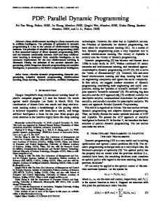
Fig. 1. A DAG Diagram.

2

DAG DATA D RIVEN M ODEL OVERVIEW

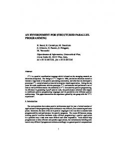
2.1 Programming Model Many applications in scientific computing consisting of a set of data or tasks with the data dependencies and precedence relationships are modeled as a Directed Acyclic Graph(DAG), such as Genome alignment, RNA secondary structure prediction, Gene finding, etc. Moreover, there are often some applications whose modeled DAG diagrams are almost the same, except for their sizes, as shown in Figure 1. In view of the reuse concept, we could make those frequently used DAGs as DAG Patterns and establish a DAG pattern library to classify and store them. Besides, lots of static and dynamic task allocation and scheduling algorithms are based on DAG. For the simplicity of parallel programming and the purpose of reusability, we could summarize one or more frequently used algorithms according to the specific application fields and implement them as code skeletons so that the programmer could call them by the arguments. Inspired by this idea, we present DAG Data Driven Model, as shown in Figure 2. It is made up of three modules: User Application Module, DAG Pattern Module and DAG Runtime System Module. The user application module presents the critical steps that the programmer needs to concern. The DAG pattern module establishes a DAG pattern library, in which lots of DAG patterns provided by system or defined by user are stored. With regard to the DAG runtime system module, it implements the static and dynamic task allocation and scheduling algorithms according to the specific applications. The three modules are closely co-related. The following are detailed descriptions of the three modules. 2.2 User Application Module The user application module is a trigger module which presents the basic steps that should be concerned and done by the programmer. It consists of five steps. According to the specific application, the programmer first chooses one DAG pattern from the DAG pattern library. If there are no suitable DAG patterns for his or her applications, he or she could define a new DAG pattern and add it into DAG pattern library. Then the next step is the DAG pattern initialization. For a selected DAG pattern, the programmer should determine its size(width, height)


3

Fig. 2. The DAG Data Driven Model Diagram.

by setting the corresponding arguments and therefore the total number of DAG nodes can be calculated. For each DAG node, the programmer should map it to the application data block. Before scheduling the DAG runtime system, some arguments must be initialized by the programmer, including input data, block size, the number of threads and the application calculation function where the programmer implements the application algorithms and functionality, etc. When the DAG runtime system starts, the application calculation function will be called by the worker threads simultaneously. All the details of parallel programming parts are transparent to the programmer, which are implemented and encapsulated in the DAG runtime system module. After computation, the final data result is returned and can be gained by the programmer. In the user application module, the programmer just needs to do some simple initialization work and focuses all of his or her attention on algorithm or functionality of the application rather than on parallelization. The common frequently used DAG patterns are stored in DAG pattern library so that the programmer could choose to use one of them by specifying the argument, which simplifies the programming and reflects the reuse concept.

By setting different sizes, we can make a DAG pattern suitable for different kinds of applications. For instance, Figure 1 is a regular DAG, and each of its nodes only depends on its left and upper nodes if they exist. It can become a DAG pattern by making its size (width and height) changeable as arguments. For a DAG pattern, each of its DAG nodes maps with a block of data, and the dependencies and relationships between the nodes could be obtained from the DAG pattern, while the computation workload for each DAG node couldn’t be obtained, which is excluded from the DAG pattern. Regarding the various application fields, we could summarize those common frequently used DAG patterns and categorize them for each field. In order to organize and manage the DAG patterns well, a DAG pattern library should be established. Each DAG pattern in the DAG pattern library has a unique identifier, by which the pattern can be selected. In the DAG pattern library, there are two types of DAG patterns, i.e. one is system provided, the other is user defined. The system provided DAG patterns are those frequently used DAG patterns summarized from the applications, while the user defined patterns, which are defined and added to the DAG library by the programmer, are the applicationspecific DAG patterns instead of the frequently used ones.

2.3 DAG Pattern Module A DAG is denoted as D={V,E}, where V={v1 ,v2 ,...,vn } is a set of n nodes, E represents the communication relationship and the precedence constraints among data nodes, and epq =(vp ,vq )∈ E represents a data message sent from data node vp to vq , which suggests that vq can start computing only after vq is completed. A DAG pattern is a regular DAG that defines the basic dependence relationships among data nodes, while its size (width,height,etc) is changeable, set by arguments.

2.4 DAG Runtime System Module The DAG runtime system module is responsible for DAG operations, parallelization and concurrency control. The runtime system adopts the master-slave pattern. Its master part is used for DAG operations, data tasks allocation and fault-tolerance control. The DAG operations include DAG parsing and updating. On one hand, the DAG parsing operation aims at discovering current new computable data nodes: it traverses every


4

Fig. 3. The computation dependency relationship and distribution of load computation density along computation shift direction. (a) and (b) are 2D/0D DP algorithms, while (c) is 2D/1D DP algorithm and (d) is 2D/2D DP algorithm.

DAG node and gets all those nodes whose in-degree is zero. By parsing the DAG, the master allocates those new computable node tasks to workers by putting the tasks into worker pool buffer. On the other hand, the DAG updating operation updates the DAG by removing those completed DAG nodes. The fault tolerance mechanism is necessary and crucial for the DAG Data Driven Model. When a computing DAG node fails, the other nodes that depend on it directly and indirectly will always be incomputable nodes. After a while, there will be no computable data nodes and the whole computation stops thereafter without any results returned. Taking Figure 1 for instance, without fault tolerance mechanism, all the nodes that depend on v(2,2) directly and indirectly will finally be incomputable nodes if the computing node v(2,2) fails unexpectedly. For the runtime system, when detecting a failed DAG node, it will re-assign the DAG node, clean the dirty results as well as workers, and recover the data computing. In order to manage the slave workers, the slave part adopts the structure of the worker pool. It has a pool buffer, which is a task interface between master and worker. The master puts the computable node tasks into it and the workers get the tasks from it. Both static and dynamic worker pools are supported here. For the static worker pool, each worker has its own buffer. The tasks and the workers are bound together according to a certain static data allocation method. Once the master puts a task into the pool buffer, the static worker pool will figure out which worker it belongs to and distributes the task to that worker’s own buffer. For the dynamic worker pool, the tasks and the workers are not bound. The workers dynamically get the data tasks from the pool buffer. If the pool buffer is not empty, all the workers must be busy working. Compared with the static worker pool, the load balancing for the

dynamic worker pool is better. The whole DAG runtime system execution process is as follows: the user application module program starts the runtime system, and the master begins to work. It first gets the user selected DAG and starts the worker pool. Thereafter, the master parses the DAG and puts the computable DAG data node tasks to the pool buffer. The worker pool allocates the tasks in the pool buffer to its workers. The worker calls the programmer’s application calculation function for computing. When a data node task is completed, the master updates and parses the DAG to find new computable DAG nodes. Once a fault is detected, the master will re-assign the data node. The whole runtime process continues until all the DAG nodes tasks are completed.

3 T HE DP A LGORITHM AND C LASSIFICATION DP is an important algorithm design technique in many scientific applications such as computational biology. It solves the problem by decomposing the problem into a set of interdependent subproblems, and using their results to solve larger subproblems until the entire problem is solved. In general, the solution to a DP problem is expressed as a minimum(or maximum) of possible alternative solutions. Each of these alternative solutions is constructed by composing one or more solutions to subproblems. If r represents the cost of a solution composed of subproblems x1 ,x2 ,...,xl , then r can be written as r=g(f(x1 ),f(x2 ),...,f(xl)), where the function g is called the composition function, and its nature depends on the problem. If the optimal solution to each problem is determined by composing optimal solutions to the subproblems and selecting the minimum(or maximum), the formulation is said to be a DP formulation[10]. Based on the dependencies between subproblems in a DP formulation, there are various classification criteria. Grama et al.[10] presents a classification of DP:


5

TABLE 1 Some Popular DP Algorithms for Computational Biology Algorithm Smith-Waterman algorithm with linear and affine gap penalty Syntenic alignment Smith-Waterman algorithm with general gap penalty Nussinov algorithm Viterbi Algorithm Double DP algorithm Spliced Alignment Zuker Algorithm CYK Algorithm

Application Genome alignment Generalized genome global alignment Genome alignment RNA base pair maximization Gene sequence alignment using HMMs, Multiple sequence alignment Protein threading Gene finding RNA secondary structure prediction RNA secondary structure alignment

DP is considered as a multistage problem composed of many subproblems. If the subproblems located on all levels depend only on the results from the immediately preceding levels, it is called serial; otherwise, it is called nonserial. There is recursive equation called a functional equation, which represents the solution to an optimization problem. If a functional equation contains a single recursive term, the DP is monadic; otherwise, if it contains multiple recursive terms, it is polyadic. Based on this classification criterion, four classes of DP are defined: serial monadic, serial polyadic, nonserial monadic, and nonserial polyadic. Considering the cache-efficient parallel execution, Chowdhury et al.[11] provide cacheefficient algorithms for three different classes of DP: LDDP (Local Dependency DP) problem, GEP (Gaussian Elimination Paradigm), and Parenthesis problem, each of which embraces one class of DP applications[12]. In this paper, we consider another classification method. That is, the DP algorithms can be classified in terms of the matrix dimension and the dependency relationship of each cell on the matrix[27]: A DP algorithm is called a tD/eD algorithm if its matrix dimension is t and each matrix cell depends on O(ne ) other cells. If a DP algorithm is a tD/eD algorithm, it takes time O(nt+e ) provided that the computation of each term takes constant time. For example, three DP algorithms are defined as follows: Algorithm 1. (2D/0D): Given F[i,0] and F[0,j] for

′

Time complexity O(n2 )

Reference [17]

O(n2 ) O(n3 )

[18] [17]

O(n3 ) O(n2 )∼O(n4 )

[19] [19]

O(n4 ) O(n3 ) O(n3 )∼O(n4 ) O(n3 )∼O(n4 )

[20] [21] [22] [19]

′

where 0≤i 0) creasing function, thereby we have the optimal minimal value S when b = d. In this case, the where ε(ε > 0) represents a small extra necessary delayed optimal minimal value S is: time for fault tolerance mechanism. Proof. In the EasyPDP, the cost of a DAG node task consists of two parts: computation cost (Cij for short) and (ii). In the case when t0 > 1, we can make ∂S ∂b = 0, waiting cost (Wij for short) in pool queue. then it has (i). The optimal value of timeout should equal to the s maximum cost of all DAG node tasks by adding a c0 × d b= (10) small extra necessary delayed time ( ε for short, (ε > k × t0 × (t0 − 1) 0)) for fault tolerance mechanism. That is, In this case, the optimal minimal value S is: p r = max√ {Cij + Wij + ε}. (19) √ t0 × (t0 − 1) × c0 × d × k + d × k × t0 0≤i,j< db S= + t0 p Next, we first prove the optimal value of c0 × (t0 − 1) + c0 × d × k × (t0 − 1) (11) r = max√ {Cij + Wij } (20) (iii). In terms of (i) and (ii), we therefore obtain 0≤i,j< db S = d × k + c0

(9)


12

at most t + 1 computable DAG nodes at any q d time when t < b .

from the ideal theoretic aspect without considering the necessary delayed time for fault tolerance mechanism. (21) (1). r ≮ max0≤i,j max0≤i,j