dynamic convex domain, so that the bound is better matched to the local curvature of the objective function, resulting in accelerated convergence. We test the ...
Parallel Majorization Minimization with Dynamically Restricted Domains for Nonconvex Optimization
Yan Kaganovsky∗ Duke University
Ikenna Odinaka∗ Duke University
David Carlson Columbia University
Abstract
where F (θ; xm , ym ) represents the data-mismatch for the mth data point (xm , ym ) ∈ Rp × Rd and θ ∈ Rp are the parameters (latent variables) to be learned. fm is a twice continuously differentiable function R → R (possibly nonconvex) that depends on ym . Here R represents a penalty due to prior knowledge (e.g., the 2norm penalty) that is separable and twice continuously differentiable (possibly non-convex). The class of optimization problems in (1) appears in various fields such as machine learning, signal/image processing, imaging and bioinformatics, to name a few.
We propose an optimization framework for nonconvex problems based on majorizationminimization that is particularity well-suited for parallel computing. It reduces the optimization of a high dimensional nonconvex objective function to successive optimizations of locally tight and convex upper bounds which are additively separable into low dimensional objectives. The original problem is then broken into simpler and parallel tasks, while guaranteeing the monotonic reduction of the original objective function and convergence to a local minimum. This framework also allows one to restrict the upper bound to a local dynamic convex domain, so that the bound is better matched to the local curvature of the objective function, resulting in accelerated convergence. We test the proposed framework on a nonconvex support vector machine based on a sigmoid loss function and on nonconvex logistic regression.
1
Often, these problems can be of huge size (large p) and involve big datasets (large M ). There is a growing need for faster algorithms that can deal with large problems in a numerically efficient way. The availability of high performance multi-core computing platforms makes it increasingly desirable to develop parallel optimization methods.
Introduction
We consider the following optimization problem θ∗ = arg min C(θ), θ∈ΩF
(1)
where ΩF is a closed convex set and C is generally non-convex and has the following form C(θ) =
M X
F (θ; xm , ym ) + λR(θ)
M X
fm (θT xm ) + λR(θ),
m=1
=
Lawrence Carin Duke University
(2)
m=1
* Indicates equal contributions. To appear in the Proceedings of the 19th International Conference on Artificial Intelligence and Statistics (AISTATS) 2016, Cadiz, Spain. Copyright 2016 by the authors.
A general optimization principle that often leads to parallelizable algorithms is majorization-minimization (MM) (Lange, 2000), also known as optimization transfer. The idea is essentially to replace a difficult optimization problem by a sequence of simpler problems. At each iteration, the original objective function is approximated by a locally tight upper bound surrogate so that minimizing the surrogate ensures that the objective function is decreased. The motivation for using MM can be to simplify the optimization process, make it more suitable for parallel computing, or both. The global convergence of this type of algorithms has been established for several cases (Lanckriet and Sriperumbudur, 2009; Mairal, 2015; Ahn et al., 2006; Jacobson and Fessler, 2007). Various well known approaches can be interpreted from an MM point of view, such as expectation-maximization (EM) algorithms in statistics (Dempster, 1977; Neal and Hinton, 1998) and difference-of-convex programming (Lanckriet and Sriperumbudur, 2009). The MM procedure has been successfully used in tomographic imaging (Ahn et al., 2006; Kaganovsky et al., 2015), image processing (Sotthivirat and Fessler, 2002), and matrix factorization (Lee and Seung, 2001), to name a few.
Parallel Majorization Minimization with Dynamically Restricted Domains for Nonconvex Optimization
A related principle is Successive Convex Approximations (SCA) (Razaviyayn et al., 2013; Razaviyayn et al., 2014), where as opposed to MM, the surrogate is not necessarily a global upper bound of the objective so that the monotonic reduction of the objective is not guaranteed. However, due to additional assumptions such as Lipchitz smoothness, convergence can be guaranteed if the step sizes are chosen to satisfy certain criteria related to the Lipchitz constant of the gradient. Well known examples that use this approach are gradient-based proximal methods (Beck and Teboulle, 2009; Combettes and Pesquet, 2011). Recently, Razaviyayn et al. (2014) proposed an SCA method for non-convex optimization where one updates blocks of variables in parallel (PSCA) while still guaranteeing convergence.
coordinate descent algorithms, where blocks are updated simultaneously on different processors while still automatically guaranteeing the reduction of the original objective function. Each of the blocks can be reduced to a small enough size such that second-order methods are practical and can be used to accelerate convergence. • The proposed method can be used with an arbitrary block size. This enables more flexibility to better explore the trade-off between convergence rate per iteration, and the time per iteration (including parallization costs such as communication between different processors), at the price of a more restrictive class of problems than Razaviyayn (2014). Note that the method by Razaviyayn (2014) is practically limited to small block sizes since it requires computing the lowest eigenvalue of the feature/system sub-matrix corresponding to each block, which becomes computationally expensive as the block size increases.
A class of parallelizable MM algorithms using partitioned-separable paraboloidal surrogates for nonconvex optimization was proposed by Erdogan and Fessler (1999) and also Sotthivirat and Fessler (2002). In this approach, the objective is approximated by a high-dimensional quadratic global upper bound and then an additional upper bound is created by using Jensen’s inequality to obtain a block coordinate descent algorithm. This approach allows one to update blocks of variables in parallel while still guaranteeing the monotonic decrease of the original objective and also convergence. A limitation of this method is that it relies on positivity constraints to construct the quadratic upper bound.
• We derive guarantees for global convergence of the proposed class of algorithms. • We test the proposed framework on nonconvex support vector machines based on a sigmoid loss function (similar to the “ramp-loss” used by Ertekin et al. (2011)) and on logistic regression with nonconvex penalties (Mairal, 2015). • The proposed method is shown to yield comparable or superior classification accuracy relative to many prior methods for non-convex optimization such as PSCA, and popular stochastic optimization methods, e.g., AdaGrad, and RMSProp.
The contributions of this work are as follows: • We propose a new type of parallelizable local majorization-minimization (MM) for nonconvex optimization which uses successive optimizations of convex surrogates. The domain of the surrogate is controlled at each iteration to better match it to the local curvature of the objective function, resulting in accelerated convergence. • Similar to Erdogan and Fessler (1999) and Sotthivirat and Fessler (2002), and in contrast to Razaviyayn (2014), our method guarantees monotonic decrease of the objective function. This has the advantage that deviation from monotonicity serves as indication of error in the code. • In contrast to Erdogan and Fessler (1999), Sotthivirat and Fessler (2002), and Razaviyayn (2014), our method uses surrogates that are matched to a local compact region of the objective function rather than globally. Also, in contrast to the first two methods, our method does not require positivity constraints. • The proposed method leads to parallel block
2 2.1
Majorization Minimization with Dynamically Restricted Domains Overview of Majorization Minimization
We begin with some basic definitions of the majorization-minimization procedure (MMP) that will be considered in this paper. Unless otherwise stated, all functions are Rp → R. ˆ ΩM ) is said to be a local firstDefinition S(θ; θ, order surrogate of a function C around an expansion point θˆ if the following conditions are satisfied ˆ ≥ C(θ) S(θ; θ) ˆ θ) ˆ = C(θ), ˆ S(θ;
∀θ ∈ ΩM ,
∇θ S|θ=θˆ = ∇θ C|θ=θˆ, ΩM ∩ ΩF 6= ∅, θˆ ∈ Int(ΩM ),
(3) (4) (5) (6) (7)
Yan Kaganovsky∗ , Ikenna Odinaka∗ , David Carlson, Lawrence Carin
where ΩM is called the majorization domain, Int(·) denotes the interior of a set and ΩF is the feasible set ˆ is also convex in the original problem in (1). If S(θ; θ) with respect to θ on some convex set containing ΩM , it is said to be a convex local first-order surrogate. The condition in (3) states that S is an upper bound of C in ΩM . The conditions in (4)–(5) state consistency of the values of the functions and their gradients at the ˆ Condition (6) is added to ensure expansion point θ. that a feasible solution exists. The condition in (7) ensures that θˆ is in ΩM and not a boundary point. The basic idea in MMP is to replace the hard problem in (1) by a sequence of easier subproblems (t)
(t)
θ(t+1) ∈ arg min{S(θ; θ(t) , ΩM ) : θ ∈ ΩF ∩ ΩM }, (8) θ
ˆ ΩM ) is the surrogate for the cost function where S(θ; θ, C in (1) with the expansion point θˆ chosen according to the last iteration θˆ = θ(t) and the majorization do(t) main ΩM = ΩM can also change with iteration. Also note that we do not require S to be strongly convex, so it can have multiple minima; accordingly, in the definition of (8) we use ∈ instead of equality. This MM procedure is guaranteed to decrease the original objective function (or leave it unchanged) if the surrogate is decreased (or unchanged), since C(θ(t+1) ) ≤ S(θ(t+1) ; θ(t) ) ≤ S(θ(t) ; θ(t) ) = C(θ(t) ), (9) where the first inequality follows from (3), the second inequality follows from (8) and the equality follows from (4). We will also show in Sec. 3 that under some mild conditions, this procedure is guaranteed to converge to a local minimum of C. The definition in (3)–(7) includes, as a special case, the paraboloidal surrogates used by Erdogan and Fessler (1999) and also Sotthivirat and Fessler (2002), where the feasible set is assumed to be ΩF = Rp+ , the majorization is on the entire feasible region ΩM = ΩF and the surrogate S is restricted to a particular quadratic form. However, to the best of our knowledge, the possibility of changing the majorization domains s.t. ΩM ⊂ ΩF has not been significantly explored. It should be noted that this idea has been mentioned by Jacobson and Fessler (2007), albeit without any specific algorithm that actually uses this approach. As we shall show below, there are important practical advantages to using local convex surrogates with dynamic majorization domains. 2.2
Convex Local Majorization
The first step of our MM procedure is to construct a convex local first-order surrogate to the noncon-
vex cost function by utilizing the specific structure in (2). Specifically, our approach relies on the observation that in most models of the form in (2) the scalar functions fm and R and their derivatives are given in closed-form. Thus, we first construct a convex surrogate for the scalar functions fm (z), where later we will substitute z = θT xm . We note that since the set of functions fm generally depend on ym they can be different for different m. Let fm : R → R be a twice continuously differentiable nonconvex function with its second derivative bounded below, i.e., ′′ min fm (z) > −∞
∀m,
(10)
′′ where fm is the second derivative of fm . Define the minimum second derivative on the interval [am , bm ]
cm (am , bm ) :=
min
am ≤z≤bm
′′ fm (z).
(11)
We now define f¯m as f¯m (z; zˆ) := fm (z) + [−cm (am , bm )]+ (z − zˆ)2 /2, (12) where [x]+ = max(0, x). It is easy to verify that for any particular m, the function f¯m (z; zˆ) in (12) is a global first-order surrogate for fm (z) (see definition in Sec. 2.1), i.e., f¯m (z; zˆ) ≥ fm (z) with equality at z = zˆ ′ ′ ′′ and f¯m = fm at z = zˆ. Also, convexity, i.e., f¯m ≥ 0, is guaranteed only on the domain [am , bm ], so in accordance with the definitions in Sec. 2.1, to obtain a convex surrogate the majorization domain should be chosen as ΩM = {θ | am ≤ θT xm ≤ bm , ∀m}. Note that for (am , bm ) = (−∞, ∞), [−cm (am , bm )]+ in (12) equals the absolute value of the global minimum of ′′ if the minimum is negative and zero otherwise, fm so f¯m in (12) is convex on the entire real line. Figure 1 illustrates the need for the local surrogate introduced in (12) and why one should consider choosing am > −∞ and bm < ∞. When the expansion ′′ > 0), adding point zˆ is located at a convex region (fm ′′ 2 [− minz∈R fm (z)]+ (z − zˆ) to the function fm (z) can lead to very high positive curvature of the surrogate and to small steps when minimizing the surrogate using second-order methods. In order to achieve faster convergence, we restrict the surrogate to the interval [am , bm ] and choose cm in (11) according to the local ′′ minimum of fm (if it is negative), which can result in a much lower curvature of the surrogate. The proposed modification leads to wider surrogates which enable taking larger steps (if needed) when using second-order methods, as illustrated by the red curve in Fig. 1. In fact, if [am , bm ] is contained in a convex region, then the quadratic term in (12) is dropped and the original function can be used in this region. To appreciate the difficulty in choosing the majorization domains ΩM or [am , bm ], note that the Hessian
Parallel Majorization Minimization with Dynamically Restricted Domains for Nonconvex Optimization Global Upper Bound
(3)–(5)) for F on the majorization domain ΩM := {θ | am ≤ θT xm ≤ bm , ∀m} when am , bm are chosen such that θˆ ∈ Int(ΩM ). (See proof in supplementary material).
Minimizing the Surrogate
Local Upper Bound
Expansion point Majorization Domain
Figure 1: Illustration of first-order convex global (blue) and local (red) surrogates for a nonconvex cost function (black). The minimum of the local surrogate is seen to be closer to the minimum of the nonconvex function than the global surrogate. All surrogates are constraint to have the same function value and gradient as the nonconvex function at the expansion point. of the nonconvex objective in (2) with respect to θ has the form H(θ) = XΛ1 X T + λΛ2 , where X ∈ Rp×M is the column-wise concatenation of the vec′′ tors xm for different m, Λ1 = Diag({fm (θT xm )}M m=1 ) M with Diag({vm }m=1 ) denoting a diagonal matrix in which the entries on the main diagonal are specified by v1 , v2 , ..., vM , and Λ2 is the Hessian of the penalty term. Accordingly, it is generally possible that a local minimum point θmin , where H(θmin ) � 0, can also sat′′ T isfy fm (θmin xm ) < 0 for some m. Therefore, choosing [am , bm ] in (12) is not a trivial task as solutions with ′′ fm < 0 must also be allowed. We propose a principled approach to tackle this problem in Sec. 4. Based on the scalar surrogates in (12), we construct a multivariate convex surrogate to a function of the P form m fm (θT xm ) (see (2)) by substituting zm = θT xm ,
zˆm = θˆT xm ,
(13)
for each m separately, where zm and zˆm are the current and reference values of the argument of fm , respectively. This is summarized in the following lemma. P T Lemma 2.1 Let F (θ) = m fm (θ xm ) with fm a twice continuously differentiable (possibly nonconvex) function. Define ˆ := F (θ) + 1 (θ − θ) ˆ T XDX T (θ − θ), ˆ F¯ (θ; θ) 2
(14)
where θˆ ∈ ΩF is an expansion point, X ∈ Rp×M is a matrix with the mth column equal to xm and D is a diagonal matrix D := Diag({[−cm (am , bm )]+ }M m=1 ),
(15)
where cm (am , bm ) is defined in (11). The function ˆ is a convex local first-order surrogate (see F¯ (θ; θ)
F¯ in (14) is generally not convex outside ΩM . In order to allow the use of any general algorithm for convex functions, we extend the surrogate to be globally convex. This extension will also be essential for our decomposition method in Sec. 2.3 that relies on Jensen’s inequality and requires the function to be globally convex. First, we introduce an extension to f¯ from (12) in ′ ′′ Eq. (16) (see next page), where f¯m (z; zˆ) and f¯m (z; zˆ) ¯ denote the first and second derivatives of fm with respect to z. Note that f˜m in Eq. (16) is globally convex even in regions where it is not an upper bound of fm and it is also twice continuously differentiable. The extension of F¯ from (14) can now be written as ˆ = F˜ (θ; θ)
X
f˜m (θT xm ; θˆT xm ).
(17)
m
The proposed MMP with Dynamically Restricted majorization Domains (DRD) is summarized in Algorithm 2.1. It is important to note that it is not necessary to solve the surrogate subproblem in (8) exactly. It is sufficient just to decrease the value of the surrogate which will result in the decrease of C in (1). Since the surrogate is a local approximation of C it might explore a small region in θ space and it is more beneficial to re-expand the surrogate at a new point than to minimize the current surrogate exactly. In addition, the extra constraint due to ΩM in (8) might make the problem more difficult to solve. Instead, we first minimize the surrogate in Algorithm 2.1 without constraining the solution to lie inside the majorization domain ΩM and then check if it lies in ΩM . If not, we project the solution to the boundary of ΩM along the line connecting the current solution θ(t+1) and the previous one θ(t) . The following lemma asserts that this projection always exists and necessarily leads to a decrease of the surrogate which implies the decrease of C. We also note that ΩM can be modified as needed, so in cases where these projections slow down the convergence, one can expand ΩM to allow larger step sizes. Lemma 2.2 Let ΩF and ΩM be non-empty convex sets with ΩF ∩ ΩM 6= ∅ and ΩM := {θ | am ≤ θT xm ≤ bm , ∀m}. Let θ1 ∈ ΩF ∩ ΩM and let θ2 ∈ ΩF with θ2 ∈ / ΩM s.t. F (θ2 ) < F (θ1 ) with F a convex function. In addition, assume am , bm are chosen such that θ1 ∈ int(ΩM ). Then there exists λ ∈ (0, 1) s.t. θ∗ := λθ2 + (1 − λ)θ1 satisfies θ∗ ∈ ΩF ∩ ΩM . Furthermore, any such point satisfies F (θ∗ ) < F (θ1 ). (Proof is provided in the supplementary material).
Yan Kaganovsky∗ , Ikenna Odinaka∗ , David Carlson, Lawrence Carin
f˜m (z; zˆ) :=
�
′ ′′ f¯m (am ) + f¯m (am )(z − am ) + f¯m (am )(z − am )2 /2, z < am ¯ fm (z; zˆ), am ≤ z ≤ b m f¯m (bm ) + f¯′ (bm )(z − bm ) + f¯′′ (bm )(z − bm )2 /2, z > bm
☞ ✎ Algorithm 2.1: MM-DRD for t ← 1 to T (or until converged) for m ← 1 to M (t) (t) Choose [am , bm ] comment: see Sec. 4 for details (t) (t) Compute c(t) m in (11) using [am , bm ] (t) (t+1) ∈ arg minθ∈ΩF {F˜ (θ; θ(t) , ΩM )} Find θ ˜ comment: F is given in Eq. (17) (t) (t) (t) Let ΩM := {θ | am ≤ θT xm ≤ bm , ∀m} (t) if θ(t+1) ∈ / ΩM then Find λ ∈ (0, 1) s.t. (t) θ∗ = λθ(t+1) + (1 − λ)θ(t) ∈ ΩM ∩ ΩF (t+1) ∗ set θ =θ return (θ(t+1) ) ✍ ✌ One practical solution to performing the projection is to use the point on the boundary of ΩM along the line connecting the previous and current solution, which has the following simple solution λ = min
(t)
bm − xTm θ(t) , T xm (θ(t+1) − θ(t) ) �M � (t) am − xTm θ(t) ∩ (0, 1) . xTm (θ(t+1) − θ(t) ) m=1
��
It should be noted that the convex surrogate in (17) can be minimized by any standard software package for convex optimization which is already more convenient than minimizing the original nonconvex cost function. 2.3
are updated simultaneously while still guaranteeing the decrease of the objective function. Since the optimization using each block potentially involves a small number of variables, it allows the use of second-order methods. Note that naively minimizing the objective with respect to blocks of variables in parallel without using the decomposition we present here would not guaranty the decrease of the objective. We can now introduce the above mentioned decomposition. Separate θ = [θ1 ; θ2 ; . . . ; θK ] into K arbitrary blocks. Define Sk as the set of all indexes used in the kth block with the corresponding variables denoted by the column vector θk and |Sk | as the number of variables in θk . We define the following function ˆ := Sm (θ; θ)
K X
k ˆ rk , xk ) Sm (θk ; θ, m m
k=1
:=
K X
k ˜ ˆT k ), rm fm (θ xm + (θk − θˆk )T xkm /rm
Jensen-Type Decomposition for Parallel Block Coordinate Descent
As shown in Sec. 3, a necessary condition for Algorithm 2.1 to converge is that the surrogate is decreased. This requires one to repeatedly evaluate the surrogate in order to determine the step-size (line-search). However, for high dimensional problems, with a large number of variables and data points, this operation is extremely time consuming. In order to alleviate this difficulty, we make use of a powerful decomposition procedure that is based on Jensen’s inequality (Boyd and Vandenberghe, 2004) and originally proposed by De Pierro (1994) that results in a surrogate that is additively separable with respect to blocks of variables (Erdogan and Fessler, 1999). This leads to a parallel block coordinate descent algorithm where all blocks
(19)
k=1
where f˜m is defined in (16), xkm ∈ R|Sk | is a subset of k xm corresponding to θk and rm is defined as k rm = kxkm k1 /kxm k1 .
(18)
(16)
(20)
Note that Sm is an additively separable function with k respect to the blocks (Sm corresponds to the kth block), so it naturally leads to a parallel block coordinate descent approach where all blocks are updated simultaneously while still guaranteeing the decrease of the objective function. P ˆ with Sm Lemma 2.3 The function S := m Sm (θ; θ) defined in (19) is a twice continuously differentiable convex local first-order surrogate (see (3)–(5)) P for F = m fm (θT xm ) on the majorization domain ΩM := {θ | am ≤ θT xm ≤ bm , ∀m} when am and bm are chosen such that θˆ ∈ int(ΩM ). (Proof is provided in the supplementary material). Remark The function in (19) is a surrogate for F on ΩM only if f˜ is globally convex since Jensen’s inequality only holds in this case. More specifically, consider k the argument of f˜m (θˆT xm +(θk −θˆk )T xkm /rm ) and note that the argument can be outside of [am , bm ] even if θ ∈ ΩM , so in that case, Jensen’s inequality would not hold if f˜ was not convex outside [am , bm ]. This provides another motivation for (16). It is worth noting that for a smaller number of groups K, the surrogate in (19) will be a tighter bound to
Parallel Majorization Minimization with Dynamically Restricted Domains for Nonconvex Optimization
✎ ☞ Algorithm 2.2: Parallel Block CD for k ← 1 to K (In parallel) (t+1) (t) θk ∈ arg minθk ∈ΩkF {S(θk ; θ(t) , ΩM )} P comment: S = m Sm comment: Sm is given by Eq. (19) ✍
✌
the original objective function with the trivial case of Sm (θ) ≡ f˜m (θT xm ) for all m when K = 1. Decreasing K will also result in harder optimization problems involving more variables for each group. On the other hand, increasing K leads to better parallelization, while resulting in a less tight bound, which can slow down the convergence per iteration but can also reduce computation time per iteration. Note that in this approach, there is complete freedom to choose any group size and to explore the above tradeoff according to the available computational resources. The resulting block-coordinate algorithm is described by Algorithm 2.1 by replacing the minimization of F˜ by the minimization described in Algorithm 2.2 where ΩkF is the projection of ΩF onto the subspace of θk . We call this algorithm Parallel MajorizationMinimization with Dynamically Restricted Domains (PMM-DRD).
3
Convergence Analysis
In order for the proposed iterative procedure to be generally useful, it must converge to a local optimum or a stationary point from all initialization states without exhibiting divergence or oscillation. To understand this analysis, we first introduce the notion of a pointto-set mapping. A point-to-set map A from a set X into a set Y is defined as A : X → M(Y ), which assigns a subset of Y to each point of X, where M(Y ) denotes the power set of Y . Next, we introduce several definitions related to the properties of point-to-set mappings. A point-to-set map is said to be closed at x ∈ X if x(t) → x as t → ∞ with x(t) ∈ X and y (t) → y as t → ∞ with y (t) ∈ A(x(t) ) implies y ∈ A(x). A point-to-set map is said to be closed on W ⊂ X if it is closed at every point of W . A fixed point of the map A is a point x for which x = A(x). A generalized fixed point of a map is a point x for which x ∈ A(x). A is said to be monotonic with respect to φ whenever y ∈ A(x) implies φ(y) ≤ φ(x). Many iterative algorithms (including the ones presented here) can be described using this notion of point-to-set maps. Let X be a set and x(0) ∈ X a given initial point. Then an algorithm A with initial point x(0) is a point-toset map A : X → M(X) which generates a sequence (t+1) {x(t) }∞ = A(x(t) ), t = 0, 1, 2, . . . . t=1 via the rule x
A is said to be globally convergent if for any chosen initial point x(0) , the sequence {x(t) }∞ t=1 converges to a point for which a necessary condition of optimality holds. The property of global convergence expresses, in a sense, the certainty that the algorithm works. It is important to stress the fact that it does not imply (contrary to what the term might suggest) convergence to a global optimum for all initial points x(0) . We analyze Algorithm 2.1 using the above tools. We start by stating Zangwill’s global convergence theorem (Zangwill, 1969, Convergence theorem A page 91). Theorem 3.1 (Zangwill, 1969) Let A : X → M(X) be a point-to-set map that given a point x0 ∈ (t+1) X generates a sequence {x(t) }∞ ∈ t=1 through x (t) A(x ). Also, let a solution set Γ ⊂ X be given and 1. All points {x(t) }∞ t=1 are in a compact set W ⊂ X. 2. There is a continuous function φ: X → R s.t. (a) x(t) ∈ / Γ ⇒ φ(y) < φ(x(t) ), ∀y ∈ A(x(t) ) (b) x(t) ∈ Γ ⇒ φ(y) ≤ φ(x(t) ), ∀y ∈ A(x(t) ) (c) A is closed at x(t) if x(t) ∈ /Γ Then all limit points1 of {x(t) }∞ t=1 are in Γ. Furthermore, limt→∞ φ(x(t) ) = φ(x∗ ) for all limit points x∗ . The general idea in showing the global convergence of an algorithm A is to invoke Theorem 3.1 by appropriately defining φ and Γ. For an algorithm that solves the minimization problem min{f (x) : x ∈ Ω}, the solution Γ is usually chosen to be the set of corresponding stationary points and φ can be chosen to be the objective function itself if it is continuous. Our approach would be to define Γ as the set of generalized fixed points and then use the fact that any generalized fixed point is also a stationary point, as established by the lemma below. Lemma 3.2 Suppose x∗ is a generalized fixed point of A described by Algorithm 2.1 (or Algorithm 2.1 with the minimization of F˜ replaced by Algorithm 2.2). Assume that the constraints as specified by ΩF in (1) are qualified at x∗ . Furthermore, assume that ΩF = {gi (θ) ≤ 0, hj (θ) = 0, i = 1, ..., I, j = 1, ..., J} where gi (θ) and hj (θ) are differentiable convex functions. Then, x∗ is a stationary point of the program in (1). (See proof in the supplementary material). We are now ready to state our main result. Theorem 3.3 (Global convergence) Let {θ(t) }∞ t=1 be any sequence generated by the algorithm described by 1 A limit point is defined as the limit of a convergent subsequence.
Yan Kaganovsky∗ , Ikenna Odinaka∗ , David Carlson, Lawrence Carin
✎ Algorithm 4.2: Localize(z, β, P) if z < � P[1] a = −∞ b = (1 − β)z + βP[1] else � if z > P[end] b=∞ a = (1 − β)z + βP[end] else Find i s.t. P[i] < z < P[i + 1] a = (1 − β)z + βP[i] b = (1 − β)z + βP[i + 1] return (a, b) ✍
Algorithm 2.1 (or Algorithm 2.1 with the minimization of F˜ replaced by Algorithm 2.2) using any initialization point θ(0) ∈ ΩF . Assume ΩF in (1) is closed and bounded and given by ΩF = {gi (θ) ≤ 0, hj (θ) = 0, i = 1, ..., I, j = 1, ..., J} where gi (θ) and hj (θ) are differentiable convex functions. Assume f and R in (2) are twice continuously differentiable functions. Then assuming suitable constraint qualifications (given by ΩF and ΩM ), any sequence {θ(t) }∞ t=1 has a limit point which is a stationary point of the program in (1), i.e., it satisfies the first-order KKT optimality conditions (Proof is provided in the supplementary material).
4
Choosing the Majorization Domains
Here we describe the algorithm for choosing the majorization domains [am , bm ] in (11). A preprocessing step involves storing all the inflection points Im = ′′ {z | fm (z) = 0}, points with minimum negative 2nd ′′ ′′ derivatives Mm = {z | z ∈ arg min fm (z), fm (z) < 0}, and the corresponding values of the second derivative ′′ χm = {fm (z)|z ∈ Mm }, for each m = 1, 2, . . . , M . We denote Mm [q] as the qth element in the ordered set {Mm [q]}Q q=1 consisting of elements of Mm and satisfying Mm [1] ≤ Mm [2] ≤ .... ≤ Mm [Q]. We define a similar ordered set for I. For simplicity, we assume that χm is a singleton set, but Mm can still contain multiple points. Algorithm 4.1 describes the procedure for selecting the majorization domain, where two parameters 0 < α, β < 1 need to be chosen. For each m, Algorithm 4.1 returns an interval [am , bm ] for which the minimal curvature is computed and used in (11). An example for using this procedure is shown in the supplementary material. In case there are multiple local minimum values of f ′′ (z), i.e., χm contains multiple different values, Algorithm 4.1 is repeated for each minimum value, after which [am , bm ] are obtained by taking the intersection of all the majorization domains. ✎ ☞ Algorithm 4.1: Domains(α, β) for m ← 1 to M am = −∞ b m =∞ Compute zm = θT xm ′′ Compute ψm = fm (zm ) if 0 < |ψ | < α|χ | m m comment: shallow region [am , bm ] = Localize(zm , β, Mm ) if α|χ m | ≤ ψm ≤ |χm | comment: medium curved convex region [am , bm ] = Localize(zm , β, Im ) return ({am , bm }M m=1 ) ✍ ✌
5
☞
✌
Numerical Results
As an application of our proposed framework for nonconvex optimization, we consider two binary linear classification problems that follow the general form in Eq. (2). The first example we consider is the sigmoidloss linear support vector machine (SVM). Standard SVM utilizes a hinge loss function as a surrogate to the 0-1 loss, which is easier to optimize and introduces a margin that allows good generalization. However, to retain a convex loss function it overly penalizes examples with large negative margins. To remedy this, Ertekin et al. (2011) proposed a ramp loss function (difference of two hinge functions). The sigmoid loss considered here is a smooth version of the ramp-loss and is given by ℓ(α) = 1 − tanh(α) (see Fig. 1 in the supplementary material). The second example we consider is logistic regression with a log penalty (Mairal, 2015) that produces sparser solutions than the L1 penalty but makes the overall problem non-convex. The regularizer is given by � Pp−1 R(θ) = λ j=1 log θj2 + ǫ where ǫ > 0 is chosen to prevent the log penalty from blowing up when θj = 0. We compare the proposed method PMM-DRD, which is described by Algorithm 2.1 with Algorithm 2.2 replacing the minimization therein, against previously proposed methods in the literature for solving nonconvex optimization problems such as Gradient Descent, L-BFGS (Schmidt, 2005), RMSProp (Tieleman and Hinton, 2012), AdaGrad (Duchi et al., 2011), and PSCA (Razaviyayn et al., 2014). We also compare to the case where the proposed method does not use restricted majorization domains, denoted PMM. In the following examples we consider binary classification tasks of distinguishing between digits 3 and 5 in the MNIST2 dataset, newsgroups 1 and 20 in the 20Newsgroup3 dataset, and HIV positive and negative patients in the TB4 dataset. The L-BFGS algorithm 2
http://yann.lecun.com/exdb/mnist/ http://qwone.com/ jason/20Newsgroups/ 4 http://www.ncbi.nlm.nih.gov/geo/query/acc.cgi?acc=GSE39941 3
Parallel Majorization Minimization with Dynamically Restricted Domains for Nonconvex Optimization
was used with 1-fold cross validation to learn the regularization coefficient λ in (2), which was then fixed to the same value for all nonconvex optimization methods. All algorithms ran till convergence, i.e., till one of the stopping criteria were met (see supplementary material for details). Due to the possible existence of local minima in the nonconvex models, we used 10 different random initializations and presented the mean results with standard deviations. Table 1 shows the classification accuracy of the sigmoid-loss SVM on the training set. One can see that among the methods for nonconvex optimization, the highest accuracy for all datasets is achieved by PMM-DRD. For the TB dataset, PMM significantly outperforms all the other methods. Figure 2 shows the nonconvex objective vs training time for the TB dataset, where it can be seen that all methods get stuck in a bad local minimum, except for the proposed PMM. Note that the restricted majorization domain in PMM-DRD leads to a convergence speed-up by a factor & 5. Table 2 shows the classification accuracy of SVM on the test set. Table 3 shows the classification accuracy of logistic regression on the training set (see Table 1 in the supplementary material for the test set). All experiments use a 64-core machine. In RMSProp and AdaGrad we use mini-batches which are 10% of the examples. The rest of the methods use the entire dataset (batch). PMM methods use blocks of 500 features. For PMM-DRD we use (α, β) = (0.1, 0.8) in algorithm 4.1. The minimization of the surrogates in PMM methods was done using the trust region conjugate gradient algorithm (Lin, 2008). We implemented PMM in MATLAB using C/C++ mex with OpenMP
400 CG
Objective Value
Table 1: Classification accuracy (%) on the training set using SVM. LIBLINEAR (Fan et al., 2008) uses the standard linear SVM, and the other methods use the nonconvex sigmoidloss. For the latter, 10 different random initializations were used and the mean and standard deviation are presented. GD=Gradient Descent, RProp=RMSProp, AGrad=AdaGrad, PMM=Parallel Majorization-Minimization, DRD=Dynamically Restricted Domain. Method MNIST 20 News TB LIBLIN 97.13 100 86.55 LBFGS 96.92 ± 0.02 99.63 ± 0.21 65.99 ± 0 CG 96.91 ± 0.026 98.36 ± 0.72 65.99 ± 0 GD 95.13 ± 1.04 95.16 ± 5.61 65.99 ± 0 PSCA 89.23 ± 0.07 79.29 ± 0.30 65.99 ± 0 RProp 96.74 ± 0.32 99.87 ± 0.09 65.99 ± 0 AGrad 94.99 ± 0.24 81.41 ± 0.63 65.99 ± 0 PMM 97.02 ± 0.02 100 ± 0 100 ± 0 PMM97 ± 0.01 100 ± 0 100 ± 0 DRD
300
GD LBFGS PSCA
200
RMSProp AdaGrad
RMSProp
350
300
GD
100
PMM PMM−DRD
0 0
5
10
AdaGrad CG
250 0
15 20 Training Time [sec]
1
2
25
Figure 2: Objective for linear SVM with sigmoid-loss vs training time using the optimization methods mentioned in Table 1 and the TB dataset. Inset shows an enlarged view of the region inside the dashed square. Table 2: Same as Table 1 but for the test set.
Method MNIST LIBLIN 96.37 LBFGS 96.65 ± 0.05 CG 96.63 ± 0.035 GD 95.7 ± 0.67 PSCA 90.89 ± 0.07 RProp 96.38 ± 0.3 AGrad 94.99 ± 0.24 PMM 96.95 ± 0 PMM96.98 ± 0.03 DRD
20 News 77.86 77.19 ± 0.9 75.45 ± 1.873 75.82 ± 3.12 68.82 ± 0.35 81.92 ± 0.81 81.41 ± 0.63 71.81 ± 0.09 78.2 ± 0.08
TB 90.72 72.16 ± 0 72.16 ± 0 72.16 ± 0 72.16 ± 0 72.16 ± 0 72.16 ± 0 91.34 ± 0.5 91.75 ± 0
Table 3: Same as Table 1 but for Logistic regression. LIBLIN uses an L1 penalty and the rest of the methods use a non-convex log-penalty. Method MNIST LIBLIN 97.33 LBFGS 97.14 ± 0.03 CG 97.81 ± 0.11 GD 95.2 ± 1.26 PSCA 88.4 ± 0 RProp 96.74 ± 0.32 AGrad 94.54 ± 0.16 PMM 98.29 ± 0 PMM98.64 0 ± 0.01 DRD
20 News 98.48 100± 0 100 ± 0 97.82 ± 3.68 97.58 ± 0.11 100 ± 0 100 ± 0 100 ± 0 100 ± 0
TB 81.44 100 ± 0 100 ± 0 89.09 ± 0.77 53.55 ± 0 56.43 ± 17.43 56.18 ± 17.21 100 ± 0 100 ± 0
enabled. PSCA uses the cyclic version (Razaviyayn et al., 2014) with 64 processors, 40 scalar features per processor, and a learning rate that is initially 1 and decreases as 1/k 1.01 , where k is the iteration number. Acknowledgements This research was supported in part by ARO, DARPA, DOE, NGA, ONR and NSF.
Yan Kaganovsky∗ , Ikenna Odinaka∗ , David Carlson, Lawrence Carin
References K. Lange, D. R. Hunter, and I. Yang (2000). Optimization Transfer Using Surrogate Objective Functions. Journal of Computational and Graphical Statistics 9(1):1–20. G. R. Lanckriet, and B. K. Sriperumbudur (2009). On the Convergence of the Concave-Convex Procedure. Advances in Neural Information Processing Systems 22:1759–1767. J. Mairal (2015). Incremental MajorizationMinimization Optimization with Application to LargeScale Machine Learning. SIAM Journal on Optimization 25(2):829-855. S. Ahn, J. A. Fessler, D. Blatt, and A. O. Hero (2006). Convergent Incremental Optimization Transfer Algorithms: Application to Tomography. IEEE Trans. on Medical Imaging 25(3):283–296. M .W. Jacobson, J. A. Fessler (2007). An Expanded Theoretical Treatment of Iteration-Dependent Majorize-Minimize Algorithms. IEEE Trans. on Image Processing 16(10):2411–2422.
Neural Information Processing Systems 27:1440–1448. A. Beck and M. Teboulle (2009). A Fast Iterative Shrinkage-Thresholding Algorithm for Linear Inverse Problems. SIAM Journal on Imaging Sciences 2:183202. L. Combettes and J. C. Pesquet (2011). Proximal Splitting Methods in Signal Processing. Fixed-Point Algorithms for Inverse Problems in Science and Engineering, Springer, New York, 185-212. H. Erdogan, J. A. Fessler (1999). Ordered Subsets Algorithms for Transmission Tomography. Physics in Medicine and Biology 44(11):2835. S. Ertekin, L. Leon, and C. L. Giles (2011). Nonconvex Online Support Vector Machines. IEEE Trans, on Pattern Analysis and Machine Intelligence 33(2):368– 381. S. P. Boyd and L. Vandenberghe (2004). Convex Optimization, Cambridge University Press. A. R. De Pierro (1994). A Modified Expectation Maximization Algorithm for Penalized Likelihood Estimation in Emission Tomography. IEEE Trans. Medical Imaging 14(1):132–137.
A. P. Dempster, N. M. Laird, D. B. Rubin (1977). Maximum Likelihood from Incomplete Data via the EM Algorithm. Journal of the Royal Statistical Society: Series B 39:1–38.
W. I. Zangwill (1969). Nonlinear Programming: A Unified Approach. Prentice-Hall, Englewood Cliffs, N.J..
R. M. Neal and G. E. Hinton (1998). A View of the EM Algorithm that Justifies Incremental, Sparse and Other Variants. Learning in Graphical Models, Springer Netherlands, 355-368.
M. Schmidt (2005). MinFunc: Unconstrained Differentiable Multivariate Optimization in Matlab. Software available at http://www.cs.ubc.ca/ ~schmidtm/Software/minFunc.htm.
Y. Kaganovsky, S. Han, S. Degirmenci, D. G. Politte, D. J. Brady, J. A. O’Sullivan, and L. Carin (2015). Alternating Minimization Algorithm with Automatic Relevance Determination for Transmission Tomography under Poisson Noise. SIAM Journal on Imaging Sciences 8(3):2087-2132.
T. Tieleman, and G. Hinton (2012). Lecture 6.5RMSProp: Divide the gradient by a running average of its recent magnitude. COURSERA: Neural Networks for Machine Learning.
S. Sotthivirat and J. A. Fessler (2002). Image Recovery Using Partitioned-Separable Paraboloidal Surrogate Coordinate Ascent Algorithms. IEEE Trans. on Image Processing 11(3):306-317.
J. Duchi, E. Hazan, and Y. Singer (2011). Adaptive Subgradient Methods for Online Learning and Stochastic Optimization, Journal of Machine Learning Research 12(39):2121–2159.
D. D. Lee and H. S. Seung (2001). Algorithms for Non-Negative Matrix Factorization, Advances in Neural Information Processing Systems 13:556–562.
R. E. Fan, K. W. Chang, C. J. Hsieh, X. R. Wang, and C. J. Lin (2008). LIBLINEAR: A Library for Large Linear Classification. Journal of Machine Learning Research 9:1871–1874. Software available at https: //www.csie.ntu.edu.tw/~cjlin/liblinear/.
M. Razaviyayn, M. Hong,Z. Q. Luo (2013). A Unified Convergence Analysis of Block Successive Minimization Methods for Nonsmooth Optimization. SIAM Journal on Optimization 23(2):1126–1153.
C. J. Lin, R. C. Weng, and S. .S Keerthi (2008). Trust Region Newton Method for Large-Scale Logistic Regression. Journal of Machine Learning Research 9:627–650.
M. Razaviyayn, M. Hong, Z. Q. Luo, and J. S. Pang (2014). Parallel Successive Convex Approximation for Nonsmooth Nonconvex Optimization. Advances in