c 2006 International Press
METHODS AND APPLICATIONS OF ANALYSIS. Vol. 13, No. 2, pp. 149–156, June 2006
001
PARALLEL POWER COMPUTATION FOR PHOTONIC CRYSTAL DEVICES∗ ULF ANDERSSON† , MIN QIU‡ , AND ZIYANG ZHANG‡ Abstract. Three-dimensional finite-different time-domain (3D FDTD) simulation of photonic crystal devices often demands large amount of computational resources. In many cases it is unlikely to carry out the task on a serial computer. We have therefore parallelized a 3D FDTD code using MPI. Initially we used a one-dimensional topology so that the computational domain was divided into slices perpendicular to the direction of the power flow. Even though the speed-up of this implementation left considerable room for improvement, we were nevertheless able to solve largescale and long-running problems. Two such cases were studied: the power transmission in a two-dimensional photonic crystal waveguide in a multilayered structure, and the power coupling from a wire waveguide to a photonic crystal slab. In the first case, a power dip due to TE/TM modes conversion is observed and in the second case, the structure is optimized to improve the coupling. We have also recently completed a full three-dimensional topology parallelization of the FDTD code. Key words. Photonic crystals, the Maxwell equations, FDTD, MPI parallelization AMS subject classifications. 65Z05
1. Introduction. Photonic crystals with photonic bandgaps are expected to be key platforms for future large-scale photonic integrated circuits. They are artificial structures with the electromagnetic properties periodically modulated on a length scale comparable to a light wavelength [1, 2]. A 3D photonic crystal offers a full photonic band gap, which prohibits light propagation in all directions. A 2D photonic crystal, which only provides an in-plane band gap for one polarization, is much easier to fabricate using present techniques. Photonic crystal waveguides are essentially line defects introduced to an otherwise perfectly periodic crystal structure. In a 2D photonic crystal waveguide, light is confined in the lattice plane by the photonic band gap effect and guided in the third dimension by total internal reflection. Fig. 1 gives two examples of 2D photonic crystal and 2D photonic crystal waveguides. The feature size, i.e., the hole diameter and slab thickness, is comparable to the light wavelength (typically around 1550 nm). Three dimensional finite-difference time-domain (FDTD) [4, 3] simulations, which offer a full-wave, dynamic and powerful solution tool for solving the Maxwell equations, are widely used to design and analyze various devices in photonic crystals [4]. The fundamental ingredient of the algorithm involves direct discretizations of the time dependent Maxwell equations by writing the spatial and temporal derivatives in a central finite-difference form on a staggered Cartesian grid [4, 3]. Since most photonic crystals involve air holes and cylinder structure, the spatial discretization has to be small enough to reduce the numerical error caused by the circular material boundaries. If a is the lattice constant of the photonic crystal pattern, usually around 450 nm, the spatial discretization should be smaller than a/10. Con∗ Received
February 4, 2006; accepted for publication August 2, 2006. for Parallel Computers (PDC), Royal Institute of Technology (KTH), SE-100 44 Stockholm, Sweden (
[email protected]). ‡ Laboratory of Optics, Photonics and Quantum Electronics, Department of Microelectronics and Information Technology, Royal Institute of Technology (KTH), Electrum 229, 16440 Kista, Sweden (
[email protected];
[email protected]). † Center
149
150
U. ANDERSSON, M. QIU AND Z. ZHANG
Fig. 1. 2D photonic crystal waveguides. Air layer, 2578nm InP top cladding, 300nm, refractive index 3.17
Air hole depth
InGaAsP core layer, 522nm, refractive index 3. 35 InP bottom cladding, 600nm, refractive index 3.17
3360nm
z
N+ doped InP substrate, 4000nm, refractive index 3.14
x y
Fig. 2. Schematics of a multilayered photonic crystal waveguide. Light is injected from the left access waveguide and travels along the y-direction.
sider the following problem shown in Fig. 2, we have a multilayered two-dimensional photonic crystal pattern. The computational domain is 5.6×18×8 µm3 . The lattice constant (distance between any adjacent air holes) is 430 nm. The air hole diameter is 279 nm. The spatial discretization is 21.5 nm in all three dimensions. There are in total 81 244 800 FDTD cells and the memory required for the input material file alone can approach one Gigabyte. The total number of time steps needed for complete power transfer is around 150 000. This problem is too cumbersome to solve by serial simulations. 2. Parallelization. The General ElectroMagnetic Solver (GEMS) codes developed by the Parallel and Scientific Computing Institute (PSCI) in Sweden are written in Fortran 90, parallelized using the Message Passing Interface (MPI) and run on a variety of parallel computers [5]. The GEMS time-domain code MBfrida is a multiblock solver based on a hybrid between the FDTD method on structured grids and the finite-element time-domain (FETD) method on unstructured grids. The large number of air holes in photonic crystals and the fact that adjacent holes are so close, makes it impossible to use a hybrid grid method. The GEMS time-domain code pscyee specializes at parallel power computation for photonic crystal devices using the FDTD method only. The initial parallelization was one-dimensional and we choose to divide the computational domain only in the y-direction. This approach is justified since the waveguide itself is along the y-direction and we only need to compute the power flows through a few XZ planes (usually two, input and output). We also assume the power planes are separate enough so that each node contains no more than one power plane.
PARALLEL POWER COMPUTATION FOR PHOTONIC CRYSTAL DEVICES
Node 1
...
Node 2
...
151
Node N
z y x
Fig. 3. One dimensional division of the computational domain.
For the power computation, a discrete Fourier transform (DFT) is computed for each of the four tangential field components and each frequency at the center of each twinkle (a side of a computational cell). In order to get tangential field component values at the center of a twinkle, interpolation is needed since it is only the normal magnetic component that is represented there due to the use of a staggered grid. At the end of the time stepping, the total power flow, i.e., Poynting’s vector, is computed. For more details see [6]. To test the performance of the parallel code, we use a simple slab photonic crystal waveguide (W3PC). The computational domain is 120×470×120 cells along the x-, y- and z-directions. The discretization ∆ is 50 nm. Since the light power concentrates in the waveguide region, the power plane needs not include the whole XZ plane and is reduced to 24×114 twinkles along the x- and z-directions. Two power planes are implemented. One works as the reference (input) and the other is the transmission power plane (output). The number of frequencies used in the power computation is 201. The parallel code is tested on the Lucidor cluster, KTH. The cluster consists of 74 HP rx2600 servers and 16 HP zx6000 workstations, each with two 900 MHz Itanium 2 (McKinley) processors and 6 Gigabyte main memory. Since FDTD is a memory bandwidth limited algorithm [7], there is no point in using more than one processor per node. The network bandwidth BW (bi-directional) is 489 Mbyte/s and the latency Tlat is 6.3 ms. The total running time of the parallel code on P nodes can be estimated, for P > 1, by Tp = Tpower + Tcom + (TF DT D /P )
(1)
Tpower is the time for computing one power plane by a single node, as we have assumed one node contains no more than one power plane. Tcom is the communication time. In each time step, two messages are sent and two received containing the values of two tangential field components, and therefore the communication time can be estimated by Tcom = 4Nts (Tlat + Smessage /BW )
(2)
Nts is the number of time steps, i.e., 25 000 in this case. Since we use 64-bit precision the message size Smessage for sending two field components is Smessage = 2 · 8 · nx nz
(3)
where nx and nz are the number of FDTD cells in the x- and z-directions, respectively. TF DT D is the FDTD updating time for 25 000 time steps when the code is run entirely on one node. Since FDTD is scalable with the number of nodes P , we divide them
152
U. ANDERSSON, M. QIU AND Z. ZHANG
to get the FDTD contribution to the total running time. The (relative) speed-up of a P -node computation with execution time Tp is given by: Sp = T1 /Tp
(4)
T1 is the total running time on a single processor. For two power planes we have T1 = TF DT D + 2Tpower
(5)
Combining the previous equations, we get: Sp =
TF DT D + 2Tpower Tpower + Tcom + TF DT D /P
(6)
The computation time for the source plane is very fast and is thus excluded from the performance model. The bottleneck of the one dimensional parallelization scheme is that one node has to complete all the computation for one power plane plus a portion of FDTD loops on its own. Thus the total running time for the parallel code is always larger than Tpower and the speed-up never exceeds 2 + TF DT D /Tpower . The speed-up for a full 3D parallelization is estimated with Sp3 =
TF DT D + 2Tpower ′ Tpower /(Px Pz ) + Tcom + (TF DT D /P )
(7)
where P = Px Py Pz and Px , Py and Pz are the number of nodes along x-, y- and z-directions, respectively. We assume Py ≥ 2 so that no node takes part in the computations of more than one of the two power planes. We also have, ′ Tcom = Nts
X i=x,y,z
2 min(2, Pi − 1)lat +
16 2nj nk BW Pj Pk
(8)
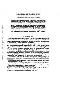
′ If we let Tcom = 0 and assume Py = 2 we get Sp3 = P . Hence, ideal speed-up is achieved if we assume infinitely fast communication between the nodes. The performance models and the measured performace for the W3PC waveguide are shown in Fig. 4. We see that the speed-up of the full three-dimensional parallelization is much better than that of the one-dimensional parallelization. Furthermore, we see that the performance models agree well with the measured values. We have also run the code with different discretization values, i.e., ∆=50 nm, 25 nm and 12.5 nm. The number of time steps has also increased accordingly (25 000, 50 000, and 100 000) to simulate the same physical process. The results, shown in Fig. 5, indicate the same power dip phenomenon (explained in the following section) with a small frequency shift.
3. Power transmissions for W1PC waveguide in 2D photonic crystals. The waveguide shown in Fig. 2 is called the W1PC waveguide, where the number “1” indicates that there is one row of missing air holes. W1PC waveguide is more widely used than W3PC waveguide as it provides a larger frequency range for lossless transmission. To inject light into this waveguide as well as to couple it out, we connect an access waveguide to both ends. The size of the access waveguide is 2500 nm along the y-direction and 750 nm along the x-direction. The power planes are placed at y=1720 nm and y=17 100 nm. The size of the power plane is 1720 nm × 6020 nm along x- and z-direction respectively. We use the commercial software Fimmwave [9]
PARALLEL POWER COMPUTATION FOR PHOTONIC CRYSTAL DEVICES
153
Predicted times for W3PC, 50nm ; Lucidor 10000 8000
t
6000 4000 2000 0
0
5
10
15 #processes
20
25
30
25
30
Predicted speed−up for W3PC, 50nm ; Lucidor 30 ideal model, px=1, py=p, pz=1 model, px=1, py=2, pz=p/2 measured, px=1, py=p, pz=1 measured, px=1, py=2, pz=p/2
speed−up
25 20 15 10 5 0
0
5
10
15 #processes
20
Fig. 4. The performance model of the parallel code. For the full parallelization we have assumed Pz = P and Px = Py = 1. W3PC
1
Transmission
0.8
0.6
0.4
0.2 ∆ = 50 nm ∆ = 25 nm ∆ = 12.5 nm 0 0.24
0.25
0.26
0.27
0.28 0.29 0.3 Normalized frequency (a/λ)
0.31
0.32
0.33
0.34
Fig. 5. Verification of the simulation on different cell sizes.
to find the eigen mode of the access waveguide and use it as the initial source. MUR first-order boundary conditions [10] are applied at the outer boundary. The total number of time steps is 150 000. The code is run on ten Lucidor nodes for 26.7 hours using the one-dimensional parallelization. Similar to the W3PC waveguide, we have observed the “mini-stop” band around 1630 nm for W1PC waveguide, as shown in Fig. 6. The power dip at this wavelength is due to the coupling between the first-order TE waveguide mode and TM mode. Since the photonic crystal only provides a bandgap for TE polarized modes, TM modes will eventually leak away in the XY plane and being absorbed by the boundaries. Towards short wavelength, around 1500 nm, the power transmission is as high as 90%. 4. Light coupling from a wire waveguide to a photonic crystal slab by generating surface modes. In this case, we study the coupling between a wire waveguide and photonic crystal slab surface modes. The structure is shown in Fig. 7.
154
U. ANDERSSON, M. QIU AND Z. ZHANG 1
0.9
Power transmission
0.8
0.7
0.6
0.5
0.4
0.3 1450
1500
1550 1600 Wavelength (nm)
1650
1700
Fig. 6. Power transmission of W1PC waveguide in 2D photonic crystal. Photonic crystal slab
Spacing S
Silicon wire waveguide
Silicon, 292nm, refractive index 3.6
Silica substrate, 2000nm, refractive index 1.45
Fig. 7. Schematics of the wire waveguide and photonic crystal slab coupling system.
The computational domain is 6.75×19.8×3.375 µm3 . The lattice constant (distance between any adjacent air holes) is 450 nm. The regular air hole diameter is 270 nm. The first five and the last five air holes on the row closest to the wire waveguide are tuned larger with diameter 288 nm in order to confine the surface modes. The air hole depth extends to the interface between silicon and silica substrate. The width of the wire waveguide is 450 nm and the thickness is the same as the photonic crystal slab (292 nm). The spacing S between the wire waveguide and the edge of the photonic crystal slab is varied for the best coupling to occur. The spatial discretization is ∆ = 22.5 nm in all three dimensions. The total number of FDTD cells is 39 600 000, which is smaller than the previous case. However, depending on the quality factor of the coupling between the waveguide mode and surface mode, the number of time step needed for this simulation can be exceedingly high. For the power computation we put two power planes 1.25 µm before and after the photonic crystal slab. The power planes center at the wire waveguide core and the area (1800 nm × 2025 nm) is smaller than the previous case because light is strongly confined in the waveguide core region for the high dielectric contrast wire waveguide. To begin with, we set the number of time steps to 200 000 and vary the spacing S.
PARALLEL POWER COMPUTATION FOR PHOTONIC CRYSTAL DEVICES
155
1
0.9
Power transmission
0.8
0.7
0.6
0.5
365nm waveguide only 500nm 275nm
0.4 Time steps = 200,000 0.3 1500
1600
1700
1800 1900 Wavelength (nm)
2000
2100
2200
Fig. 8. Power transmissions of the wire waveguide placed at different distances (S) from the photonic crystal slab edge.
The results are shown in Fig. 8. The red curve with triangular markers shows the power transmission of a stand-alone wire waveguide without photonic crystal slab beside. The green, blue and black curves correspond to the case when the spacing S = 500 nm, 365 nm, and 275 nm, respectively. In all cases, the waveguide mode couples to the slab when the wavelength goes beyond 2020 nm. For wavelengths between 1800 and 2000 nm some surface modes are generated, which are shown as the power dips. When the spacing between the wire waveguide and the photonic crystal slab decreases, strong coupling takes place. In the next step, we fix S = 275 nm and increase the number of time steps to 800 000. The wavelength region is decreased in order to give a detailed power transmission plot. More surface modes appeared for increased time steps and the power drop for the principle surface mode at 1868 nm is close to 10% The total computation resource used using the one-dimensional parallelization is twenty Lucidor nodes for 40 hours. The results are shown in Fig. 9. 5. Summary. To conclude, we have parallelized a GEMS time-domain code for power computations in photonic crystal devices. The parallel performance was not optimal when using the one-dimensional topology. Nevertheless, it allowed us to compute long-running large-scale structures which could not be handled by the serial code. Using the parallel code, we have studied the transmission property of a photonic crystal waveguide in a multilayered structure. We have also investigated the coupling between a silicon wire waveguide and a photonic crystal slab. Different coupling strength is observed for different waveguide/slab spacing and detailed power transmission spectrum is obtained for the wavelength region of interest. We have also recently completed a full three-dimensional topology parallelization of the FDTD code. 6. Acknowledgement. This work was supported by the VR project 621-20035501, the SSF project on photonics, and the computational resources of the center for parallel computers (PDC) at KTH. The module used for computing the power flow was supplied by Saab Avionics AB.
156
U. ANDERSSON, M. QIU AND Z. ZHANG 1 0.9
Power transmission
0.8 0.7 0.6 0.5 0.4 0.3 Time steps = 800,000 0.2 0.1 1835
1840
1845
1850 1855 1860 Wavelength (nm)
1865
1870
1875
Fig. 9. Detailed power transmission for spacing of S = 275 nm. The number of time steps is increased to 800 000.
REFERENCES [1] E. Yablonovitch, Inhibited Spontaneous Emission in Solid-State Physics and Electronics, Phys. Rev. Lett., 58 (1987), p. 2059. [2] T. F. Krauss, R. M. De La Rue and S. Brand, Two-dimensional photonic-bandgap structures operating at near-infrared wavelengths, Nature, 383 (1996), p. 699. [3] K. S. Yee, Numerical solution of initial boundary value problems involving Maxwell’s equations in isotropic media, IEEE Trans. Antennas Propag., AP-14 (1966), p. 302. [4] A. Taflove and S. Hagness, Computational Electrodynamics: The Finite-Difference TimeDomain Method, Artech House, Boston, MA, 2005, 3rd edition. [5] B. Strand, U. Andersson, F. Edelvik, J. Edlund, L. Eriksson, S. Hagdahl and G. Ledfeldt, Numerical solution of initial boundary value problems involving Maxwell’s equations in isotropic media, AP2000 Millennium Conference on Antennas and Propagation, Davos, Switzerland, April 9-14, 2000. [6] T. Martin, Broadband Electromagnetic Scattering and Shielding Analysis using the Finite Difference Time Domain Method, ISBN 91-7219-914-8, Link¨ oping, 2001. [7] U. Andersson, Yee bench—A PDC benchmark code, TRITA-PDC, 2002:1, KTH (2002), November. [8] G. Amdahl, Validity of the Single Processor Approach to Achieving Large-Scale Computing Capabilities, AFIPS Conference Proceedings, 30 (1967), p. 483. [9] Photon Design, Fimmwave, http://www.photond.com/products/fimmwave.htm. [10] G. Mur, Absorbing Boundary Conditions for the Finite-Difference Approximation of the TimeDomain Electromagnetic-Field Equations, IEEE Trans. Electromagn. Compat., 4 (1981), p. 377.