Parallel Processing on Supercomputers: A Set of Computational. Experiments*. N. Balram. C. Belot. J. M. F. Moura. Depart. Elect. and Comp. Eng., Carnegie ...
Parallel Processing on Supercomputers: A Set of Computational Experiments* N.Balram
C. Belot
J. M. F. Moura
Depart. Elect. and Comp. Eng., Carnegie hlellon University, Pittsburgh, PA, 15213.
Abstract
will have improved computation rates for each CPU because of advances in technology (further decrease in clock cycle times, faster memories, etc.), the major speedup will result from the availability of larger numbers of CPUs to process work in parallel. The different types of parallelism available on the Cray X-MP are vectorization, microtasking, and macrotasking, the last two often collectively referred to as multitasking. Vectorization is the process of re-. placing a block of sequential code by instructions that use vector functional units. The compiler analyzes the user program, identifies computations that can be overlapped, and produces object code to carry out these computations using the vector hardware available. On the Cray, this is presently done a t the level of the innermost DO loop. CRI'defines multitasking to be the process of dividing a program ,into segments which are then executed in parallel. This paper discusses our experiences with both forms of multitasking available on the Cray X-RIP. Vectorization issues are dealt with only when they arise in connection with multitasking. This approach is adopted because vectorization is performed automatically by the compiler and therefore requires only a little insight and care on the part of the programmer. Furthermore, well written, general references on this subject are available (see (31 ). Also, in [8] a pertinent detailed discussion on some vectorization issues, is presented. We concentrate on multitasking, instead. Section 2 deals with microtasking while section 3 discusses macrotasking, comparing and contrasting it with microtasking. Details of the actual implementation of these constructs are avoided. There is ample literature available on this (see [4], [5], [SI). The goal is to focus on the principles behind them and use experimental results to derive rules of thumb to guide other users in implementing Illultitasked progran=. ~ 1 prograins 1 discussed are coded in Fortran' Even though this paper is primarily concerned with
One of the trends in supercomputer evolution lies in the direction of multiprocessor systems with increasing numbers of powerful processors. The user who is interested in attaining the maximum achievable computation rates on these machines must understand the philosophy underlying the parallel processing mechanisms provided on them. This paper focuses on the three types of parallelism currently available on the Cray: vectorization, microtasking, and macrotasking. Experiences with all three constructs are presented with a view to exposing the improvements possible with each of them. While this paper deals with a particular machine, the Cray X-MP/48, many of the observations, comments, and conclusions derived can be generalized to other shared-memory multiprocessor systems.
1
Introduction
One of the trends in supercomputer evolution lies in the direction of multiprocessor systems with increasing numbers of powerful processors. Consider Cray as an example. The Cray-1 was introduced in 1976 as a uniprocessor system with orders of magnitude speedup over mainframes, because of its faster clock cycle, large and fast memory, and its ability to perform vector arithmetic. The Cray X-MP/2, introduced in 1982, has 2 CPUs, the Cray X-MP/4, introduced in 1984 has 4 as does the Cray-2, introduced in 1985. The trend in the next generation Cray machines is towards even larger numbers of processors: the Cray Y-MP with 8 CPUs, the Cray-3 with 16, and the Cray-4 with 64. While each of these machines 'The work reported here w a s performed using the facilities of the Pittsburgh SuPercomPUtillg Center(PSC), and SPOnsored by NSF grant # ECS-8515801 ton leave from Instituto Superior Tdcnico and CAPS, Universidade TCcnica de Lisboa, Portugal, on a fellowship from Junta Nacional de InvestigqIo Cientifica e Tecnol6gica
' Cray Research Inc.
(JNICT). 241
CH2617-9/88/0000/0247$01.00 0 1988 IEEE
the Cray X-MP architecture and tlie parallel processing structures available on it, many of the principles incorporated are general enough to be applied to other systems such as the IBM 3090, and the Alliant FX/Series, which, like the X-MP, are shared-memory multiprocessor configurations. See [l]for a coniprehensive architectural taxonomy of supercomputers. The applications discussed in this paper were run on two Cray X-MP/48 machines, one at the Pittsburgh Supercomputing Center (PSC), the other a t CRI in hlendota Heights. The Cray X-MP/48 consists of 4 independent enhanced Cray-1 processors, sharing a 32 or 64 way interleaved central memory of Shlwords (64 bit words). Each CPU has a set of address computation units, two sets of integer functional units, and one set of floating point functional units comprising of add, multiply, and reciprocal approximation. In addition, each CPU has four ports to main memory, allowing two memory reads, one memory write, and 1 / 0 to proceed siniultaneously. The Cray X-MP is a register-to-register architecture, with each processor having a set of 8 vector registers of G4 words ((34 bits/word). The clock period of the X-hlP/4S a t the PSC is 9.5 nano seconds, corresponding to a peak rate of 210 MFLOP per CPU.
2
Microtasking
Microtasking is a simple mechanism for partitioning a task into independent segments that can be processcd in parallel (see [4], [GI). Microtasking was designed to automatically do dynamic load partitioning, i.e., the work is assigned to the processors available at runtime. The idea is to stack up parallel work in independent pieces that are picked up by processors as and when they are available, instead of assigning it to specific CPUs. This eliminates time wasted when one CPU is waiting for another to return from other duties and finish processing its assigned work. Dynaniic load partitioning makes efficient use of idle CPUs i n a batch environment. hIicrot,askiiig does not involve progranmiing individual processors. It is primarily a method of controlling access of available processors to segments of code and variables in the program. This is done by inserting directives in the code. A preprocessor, called PREMULT, is invoked prior to the running of the microtasked code. It interprets the directives and rewrites the program, making calls to the microtasking library where necessary. This is transparent to the user. Since these directives appear as comment lines (they always begin with a C), they do not reduce the portability of the program. Furthermore, since tlie
successful execution of the program is independent of the actual number of processors, the code written for a particular machine, say the Cray X-MP/4, can be run efficiently on other machines with different numbers of CPUs (for example Cray X-MP/2 or Cray Y-MP). Because of its low overhead, microtasking can be used to process tasks with small granularity as well as large. In [7], it is concluded that microtasking is useful for tasks with granularity greater than 1000 clock periods, which allows it to be used at the DO loop level and sometimes even a t the statement level. The fine-granularity possible makes a bottom-up approach to parallelizing a problem/program viable. Since multitasking a program is primarily a data access problem, one of the most important steps is the analysis of the scope of the variables. A bottom-up approach simplifies the data analysis, because it is easier to analyze scope at lower levels. Bottom-up is particularly convenient when, as is often the case, most of the Computation is concentrated in a few subroutines. Microtasking allows the prograninier to esploit any parallelism in these routines, without needing to bother about tlie rest of the program. The first of our algorithms that was considered for microtasking was the two dimensional convolution. The bulk of the computational load, in many signal processing applications is concentrated in this operation. That along with the nested loop structure of tlie algorithm makes it ideal for microtasking. Figure 1 shows the two dimensional asymmetric convolution (see [8]). It has three loops nested one inside the other; often one of them is short. The optimized implementation, from tlie vectorization point of view, has the short loop unrolled (to minimize memory references) with the innermost loop being the largest one. The outer loop can be microtasked, because tlie iterations are independent of each other, and can therefore be performed by different processors in any order (see Figure 1). The unmicrotasked routine ran a t 159 AlFLOPS while the microtasked one ran at 618 MFLOPS thus providing a speedup of 3.88 (the speedup due to multitasking is defined as the ratio of the wall clock time of the unmultitasked code to the wall clock time of the multitasked code with both being run on a dedicated system). The synimetric version of the two dimensional convolution has array B(*) identical to A(*). The asymmetric code is converted into the symmetric version by replacing the B(*) array by A(*) and then pulling out the A(1) common to each pair of operands, for esainple A( 5)*XN 1(I,J+5)+B( 5)*XN 1(I,J+15) beconies A( 5) *(XN l (I ,J +5)+XN l (I ,J 15)) (see Fig-
+
CMICS DO GLOBAL DO 40 I=1.64 DO 20 J=1,512 XN(I,J)= A(5)*XNl(I,Jt5)+B(5)*XNl(I,J+15)
+A(4)*XNl(I,Jt6)+B(4)*XNl(I,J+14) t A( 3)*XN1( I,J +7)+B(3)*XNl(I, J + 13) tA(2)*XNl(I,J+8)+B(2)*XNl(I,J+l2) +~(1)*XN1(I,J+9)+B(1)*XN1(I,J+ll) 20 40
SUBROUTINE convl-A
c! -
+XNl(I,J+lO) CONTINUE CONTINUE RETURN END
DO 16 J=20,1812 P(J)=F(J) DO 15 I=1 19 P(J)=P(J)~A(I)*(F(J-I)+F(J+I)) CONTINUE CONTINUE RETURN END
15 16
Figure 1: Two-dimensional asymmetric convolution SUBROUTINE conv2-A
ure 1). The unmicrotasked two dimensional symmetric convolution ran a t 145 MFLOPS while the microtasked one ran a t 547 hiIFLOPS thereby providing a speedup of 3.78. The excellent computation rate obtained for both versions of the convolution confirms that the performance of this kind of operation is considerably enhanced by microtasking. The one dimensional convolution is another worthwhile candidate for niicrotasking, for the same reasons mentioned in the context of the two dimensional convolution. The operation requires two DO loops, one nested inside the other. Often one of the DO loops is much smaller than the other. This is the case in a program which is discussed later in this section. The numbers used in the convolution correspond to the actual numbers in production runs of that program, making it a real example rather than a cookbook one. In such cases, optimum vectorization dictates that the shorter loop be unrolled to minimize memory references. Three possible implementations are shown in Figure 2 : c o n v l (Figure 2(a)) has the smaller loop nested inside the larger one, conv2 (Figure 2(b)) has the larger one inside the smaller, convd (Figure 3(c)) is the same as conv2but has the outer loop unrolled to minimize memory references. All three were microtasked and run on a dedicated machine (see Figure 3 and Table 1). As expected, convl performed the worst in both cases (microtasked and unmicrotasked) because the inner loop is too small to provide good vector performance, and the gain in performance, as a result of microtasking is not enough to offset the loss in vectorization. The unmicrotasked vcrsion of conv2 ( c o n v 2 - A ) ran at 135 MFLOPS because of the large inner loop length (1792). Since the outer loop iterations are not independent, this could not be microtasked the way the
DO lJ=20,1812 P(J)=F(J) DO 16 I=1,19 DO 15 J=20,1812 p(J)=p(J)+A(I)*(F(J-I)+F(J+I)) CONTINUE CONTINUE RETURN END
1
15 16
SUBROUTINE conv3-A C
, , , ,
:,
, , , , ,
: :, , 1
16
DO 16 5 ~ 2 0 , 1 8 1 2 P(J)= A(lS)*(F(J-lS)+F(J+ 19)) +~(i8)*(~(~-18)+~(J+18)) +A(17)*(F(J-l7)+F(J+17)) +A( IS)*( F(J-lG)+F(J t 16)) +A(15)*(F(J-l5)+F(Jt15)) +A( 14)*(F(J-l4)+F(Jt14)) +A(13)*(F(J-l3)+F(J+13)) +A(12)*(F(J-l2)+F(J+12)) +A( 1 l ) * ( F ( J - l l ) t F ( J + l l ) ) t~(io)*(~(~-lo)+~(J+lO~) +A(S)*(F(J-S)+F(J+S)) +A(d)*(F(J-d)+F(J+S)) +A(7)*(F(J-7)+F(J+7)) +A(S)*(F(J-6)+F(J+S)) +A(S)*(F(J-S)+F(Ji-5)) +A(4)*(F(J-4)+F(J+4)) +A(3)*(F(J-3)+F(J+3)) +A(2)*(F(J-Z)+F(JtZ)) +A(l)*(F(J-l)+F(J+l)) +F(J) CONTINUE RETURN END
Figure 2: Three different implementations of the onedimensional convolution
249'
routine
wall-clock time (msI l(j3.2 conv 1-A 46.19 convl-B 15.09 ~0nv2-A 7.305 conv2-B 14.11 conv3-A 4.342 c0nv3-B
MFLOPS
CMICS MICRO SUBROUTINE convl-B CMICS DO GLOBAL DO 16 J=20,1812 P(J)=F(J) DO 15 I=1,19
Speed Up (AIBI \ .
P(J)=P(J)+A(I)*(F(J-I)+F(JtI)) 15 16
I
L
12.5 44.23 135.4 279.6G 144.8 470.5
3.53
CONTINUE CONTINUE RETURN END
2.065 CMICS MICRO SUBROUTINE conv2-B DO 1 3=20,1812 1 P(J)=F(J) L = 181214 DO 16 I=1,19 CMICS PROCESS DO 15 J=20,L P(J)=P(J)+A(I)*(F(J-I)+F(J 15 CONTINUE CMICS ALSO PROCESS DO 17 J=L+1,2*L
3.25
two dimensional convolution was. To microtask this we split the inner loop into 4 smaller loops, each of which could then be run in parallel (see con218-B, Figure 3(b)). The. resulting task granularity was too small to provide good speedup (we define 3.0 or more as good on a 4 processor system). Therefore the microtasked code ran a t 280 MFLOPS, corresponding to a speedup of 2.07 (see Table 1). As expected the unmicrotasked version of con&? (conv3-A) ran faster than either of the other two unmicrotasked versions, a t a speed of 145 MFLOPS. It has no outer loop a t all, so, as before, to microtask the routine, we broke the loop into 4 smaller loops (see conv.%B, Figure 3(c)). The task granularity was enough to allow a reasonable speedup (more than 3). The microtasked version A ran at 471 MFLOPS, a speedup of 3.25 . Increasing the loop length by an order of magnitude produced a rate of 557 MFLOPS for the microtasked code as opposed to 148 MFLOPS for the unmicrotasked, a speedup of 3.77. The reason why the strategy of breaking up the inner loop into smaller loops to be run in parallel worked so well here is that the Cray is a register-toregister architecture. This makes it possible to run even short vectors a t reasonable computation rates, i.e, the half performance length is fairly small. The half performance length, 1 1 / 2 , is defined as the lengtli of a vector for which half of the masimum performance is obtained for that operation [3]. A vector typical of the kind generated by unrolling small outer loops was run with different loop lengths, on a dedicated machine (see Figure 4). The resulting performance is plotted in Figure 4 . From the plot, it is clear that for vector lengths greater than 48 the computation rate increases very gradually, approaching 148 JiFLOPS asymptotically. Therefore, once past the knee of this curve, the best strategy is to break up the loop into smaller loops that can be run in par-
P(J)=P(J)+A(I)*(F(J-I)tF(J 17 CONTINUE CMICS ALSO PROCESS DO 18 J=2*L+1,3*L P(J)=P(J jtA(I)*(F(J-I)+F(JtI)) 18 CONTINUE CMICS ALSO PROCESS DO 19 J= 3*Lt1, 1812
P(J)=P(J)tA(I)*(F(J-I)+F(J+I)) 19 CONTINUE CMICS END PROCESS 16 CONTINUE RETURN END
CMICS MICRO SUBROUTINE conv3-B L = 181214 CMICS PROCESS DO 16 J=20,L P(J)= A(19)*(F(J-l9)tF(J+19))
, +A( l)*(F(J-l)tF(J t l ) ) I -tF(J) 16 CONTINUE CMICS ALSO PROCESS DO 17 J= L t 1 , 2*L
. . .
17 CONTINUE CMICS ALSO PROCESS DO 18 J= 2*L+1, 3*L
. . .
CONTINUE c i 4 r c s - A L s o PROCESS DO 19 J = 3*L+1, 1812 P(J)= A(lg)*(F(J-l9)+F(Jt19))
Id
END
(c) Figure 3: Microtasked versions of the 3 implementations of the one-dimensional convolution
250
allel. The degradation in performance due to smaller loop length is very small in this region (see Figure 4) while the computation rate possible, with even 2 CPUs available, will exceed that of the single larger loop run on one C P U . For example (see the table in Figure 4) a loop of length 64, which runs at 106 MFLOPS on a single CPU, can be broken into 4 loops of size 16 each of which can now run on separate processors a t 53 MFLOPS apiece giving a best case rate of 212 MFLOPS, an improvement of 100% . For larger loop lengths the improvements possible are even greater. A simple formula2 to compute the asymptotic computation rate for any vector involving only floating point additions and multiplications, and memory reads and writes is:
, , ,
, , , ,
,
,
20
,
DO 20 J = l l , N F(J)=B( lo)*( C( J-10) C( J t 10)) +B(9)*(C(J-9) C(Jt9)) +B(d)*(C(J-d) C(J+S)) +B(7)*(C(J-7) C(J+7)) tB(6)*(C(J-6) C(J+6)) +B(5)*(C(J-5) C(Jt5)) tB(4)*(C(J-4) C(Ji-4)) +B(3)*(C(J-3) C(J+3)) tB(2)*(C(J-2) C(J+2)) t B ( l ) * ( C ( J - l ) C(J+1)) +C(J) CONTINUE
MFLOPS
Loop Length
8
H
where n, is the number of floating point additions, n,, the number of floating point multiplications, m, the number of memory writes, and m,. half the number of memory reads, performed per iteration of the loop. The composition of the formula is intuitive. The (G4/G8) factor comes from the fact that a floating point unit can perform a masimum of G4 operations i n 66 clock periods. The (105) factor converts this to the number of floating point operations per second. A clock period of 9.5 nano seconds corresponds to 105 million periods per second. When using this formula for an X-MP with a different clock period, this factor will have to be changed accordingly. The remaining factor measures the overlap of the addition and multiplication functional units. For example, the two dimensional symmetric convolution has 10 adds and 5 multiplies in each iteration of the inner loop and so the overlap factor works out to be 1.5. The best case performance would be for an algorithm with an equal number of additions and multiplications thus leading to an overlap factor of 2, i.e., the add and multiply units overlap completely and in every G8 clock periods G4 adds and G4 multiplies are performed. The denominator of this factor reflects the constraints imposed by the limited number of paths between a CPU and main memory, allowing only 2 memory reads and 1 memory write to proceed simultaneously.
11.
*This formula w a s communicated to the authors by David Slowinski of Carnegie Mellon University and the Pittsburgh Supercomputing Cent er( PSC).
+
+ + + + + + + ++
16
I
.
31.15 53.4 80.97 9G.24 106.54
I
n
,
. , .
I
4000
6000
8000
.
,
20
0
2000
10000
Loop Length
(c) Figure 4: Vector performance of an example loop on a single CPU 25 I
time using the relations
Using this formula the sample loop, displayed in Figure 4, (as well as the loop in conv3 of the convolution) is computed as having an asymptotic computation rate of 148 MFLOPS. This corresponds well with the experimental results obtained . The half performance length, l l 1 2 , for this example is between 16 and 32 (see table in Figure 4) reinforcing the assertion that even moderately long (64 and above) loops of this kind should be broken into smaller loops that can run in parallel. Some general conclusions can be drawn from these experiences. We looked a t one implementation of the one-dimensional convolution, in which microtasking was substituted in place of vectorization (in convl, in which the innermost loop is the shortest one). Clearly this is not a good idea because vectorization currently provides a larger speedup than microtasking (an order of magnitude versus 4), though this could change in systems with more CPUs. The other two implementations of the one-dimensional convolution (conv2 and conv3) allowed us a less drastic choice, namely to tradeoff some vectorization performance in exchange for microtasking. This w a s done by breaking up loops into smaller ones, which could then be run, albeit a t lower vector rates, in parallel using multiple CPUs. High computation rates (up to 557 RIFLOPS) were achieved in this manner, because of the small amount of degradation in vector rates for even moderate loop lengths (see Figure 4). This approach is viable in batch environments, because an increase in c0niput.ation rate is possible with as few as two CPUs available. Finally, an application program of considerable interest to the authors’ research was considered for microtasking. It serves here the objective of testing the viability of microtasking in an actual application where decreasing the elapsed time is an important goal. To realize real-time applications this code must run considerably faster than a uniprocessor Cray XMP presently allows. One way of achieving the higher computation rates needed is by using multitasking. The computer program we are dealing with simulates the phase modulation/demodulation problem. See for example [9] for more on the physics and practical interest of the problem, and alternative considerations regarding its implementation in an array processor. The so-called point-masses filter, which a p proximates the optimum nonlinear filter with arbitrarily small error, computes the a posteriori probability density, F,,(i),(conditional density of the signal given the observations) as a sequence of masses a t discrete points, i , of a grid.This density is propagated in
where Pn+lis the prediction density, Qn is a function of the signal model, and On+l depends only on the observations a t the current time, n. The symbols * and denote convolution and pointwise function multiplication respectively. All the quantities in (3) are computed in a discrete set of grid points, although the dependence on i has been omitted. The specific grid to use depends on problem parameters such as the signal-to-noise ratio. Once the a posteriori density, Fn, is known for a particular time instant, n, signal estimates are computed according to the cost-function one wants to minimize. The algorithm (3) can be interpreted as a discretized version solution to a partial differential equation (PDE). The performance of this filter, and in general the performance of a nonlinear filter, can only be assessed by Monte Carlo methods. Signal and observations are generated for a given time set IN (e.g., = [l,2,.. . , lOOO]), the estimate being the output of the filter routine. This procedure is repeated a large number of times. As long as one guarantees i a t each repetistatistical independence bet \ v ( ~ * idata tion, meaningful statistical results can be obtained. Aside from the initialization procedures, the main program consists of a large outer (Monte Carlo) DO loop, each iteration computing a time sequence of signal estimates. The actual error for each time instant is computed as well as other parameters describing the behavior of the filter. This data is written to a file for processing. Convolution is the most computationally intensive routine in the program. This routine, along with all the other routines that can be microtasked, account for a t best 75% of the execution time. Amdahl’s law predicts that this would provide a speedup of less than 2.3, even if the microtasked code ran a t 100% efficiency, i.e., if all the microtasked segments ran 4 times faster than their unitasked versions. Instead of microtasking a t the lower level, as is usually the case, a more productive (in terms of speedup obtainable) approach is to exploit the natural parallelism of the problem, namely the almost independent Monte Carlo iterations. For the purpose of parallel execution, the main problem arises in the generation of independent paths for each Monte Carlo loop iteration. Actu-
252
the microtasked version was executed, then the two macrotasked versions one after another (they are discussed in the next section). The timing data compiled from these sessions is recorded in Table 2, with the batch runs tlistinguished by the time the session was conducted at. The best speedup obtained was 3.0G (see results in Table 2). This was computed using the wall clock timings on the dedicated machine. As predicted by Amdahl’s law the maximum speedup theoretically possible is limited by the sequential portion of the program, in this case mainly the random number generator. With the help of FLOWTRACE, an analysis tool, the percentage of execution time of the unitasked program spent in the random number generator was computed to be 5.67. The other sequential portions of the program contribute another 2.14% to this. Then Amdahl’s law predicts that the maximum speedup possible is 3.24 (100/(7.81 92.19/4) = 3.24), assuming the microtasking is 100% efficient, i.e., the microtasked segment runs 4 times faster than the original unitasked version. Note that Amdahl’s law is applicable here because the serial portion of the problcm grows along with the parallel portion when the nuniber of hlonte Carlo iterations is increased. Thus the ratio of serial to parallel portions remains constant with increasing problem size (i.e., increasing Monte Carlo iterations) unlike the kinds of problems dealt with in [2]. The actual speedup obtained (3.0G) is close to this. Using Amdahl’s law, the microtasked portion speedup works out to be about 3.7. The 1 / 0 in the Monte Carlo loop is responsible for restricting the niicrotasking segment speedup to 3.7 because it creates a critical region in the code (a critical region is one which can be accessed by only one processor a t a time, see [4]). The program could be rewritten to avoid performing 1 / 0 in the Monte Carlo loop, but the modest gain in performance (an increase in total program speedup, from 3.06 to 3.24) makes the additional labor an unattractive proposition. There is an important philosophical difference between writing a niultitasked program from scratch and converting esisting sequential code into a multitasked form. When writing a niultitasked program, the programmer can structure it so as to exploit all the natural parallelism in the problem. For most applications, however, working sequential code exists. It is more practical to multitask this, while retaining the basic structure, rather than rewriting it. Situations such as in the phase demodulation program discussed here often arise, i.e., some facet of the original program
ally, random number generators guarantee independence (more rigorously very small correlation) bet.ween numbers computed sequentially, but if a copy of the same generator is given to each task running in parallel the random numbers, and consequently the signal and the observations, would be the same for all tasks. To overcome this problem, the random generator routine can be defined as a protected region whose updates are known by every task. There are two reasons why this solution is not viable: i) the overhead due to tasks waiting to entering the critical region would be large (each observation requires 3 random numbers) in comparison with the computations; ii) the order in which microtasked loop iterations are processed is non-deterministic, varying from run to run, leading to results that are not reproducible. An alternative solution, that avoids the two problems mentioned above is to precompute all the random numbers needed and store them in a matrix. Each Monte Carlo iteration accesses the numbers it needs, stored in different columns of the matris. This makes the iterations independent. The only remaining issue is the handling of the critical regions in the loop, i.e, those places in which all the iterations make use of a shared resource. The original program was coded so as to output results during each Monte Carlo iteration. The 1/0 has to be monitored to ensure that no two tasks write to the same file at the same time. With these issues taken care of, the program was microtasked by placing the entire Monte Carlo loop inside a subroutine and then defining each iteration of the loop as a process (the smallest amount of work handled by a processor at a time). Scaled down versions (with 48 Monte Carlo iterations) of both the unmicrotasked and the microtasked programs were run on a dedicated machine as well as in a batch environment. Program esecution times (i.e., wallclock time) are consistent on a dedicated machine. In batch mode, however, the execution time depends on the load on the system and fluctuates widely from one run to another. In order to facilitate comparisons between the performance of the multitasked code and the unitasked (i,e., unmultitasked) code, with both run in batch mode, they were run in multiple sessions at different times of the day. Each session consisted of one unitasked run, one microtasked run, one macrotasked (using static partitioning), and one macrotasked (using dynamic partitioning). The programs comprising a session were run one after another, always ensuring that only one of them w a s running on the machine, a t a time. Thus for example the 10 am session began with the unitasked program. As soon as it finished executing,
+
253
inhibits full multitasking. In such cases a tradeoff is evident here in terms of time spent versus speedup obtained. A judgement has to be made whether the increase i n performance that results from the restructuring of the original program justifies the amount of time it takes to do it. The phase demodulation program could have been microtasked by simply microtasking the convolution and other amenable routines. This provided a maximum attainable speedup of 2.3, for the entire program. As discussed earlier, the restructuring of the program to precompute the random numbers before the Monte Carlo loop increased this to 3.06. The increase clearly justified the modest effort required. Further restructuring, of the 1/0 in the hIonte Carlo loop, could bring this closer to 3.24, the theoretical maximum. At this stage, the marginal improvement in performance was considered too sinall to justify the additional effort. The dedicated system timings show t,liat niicrotasking can improve the performance of this program by a factor of 3. For practical reasons, the improvement achieved i n the batch environment was considered more important. Since batch system timings vary from run to run, it is difficult to find a metric to quantify the speedup achieved through microtasking. I t makes no sense to compare the microtasked code timings with the timings of the unitasked code with the latter run on a dedicated machine. Nor is it reasonable to compare any arbitrary microtasked timing with just any unitasked timing, with both being run i n a batch environment. One reasonable way to gauge the speedups possible is by comparing the mall clock timings for the microtasked code with the timings for the unitasked code, run on a batch system, as close together as possible without having both jobs running on the system a t the same time (i.e., the jobs run in the same session are compared). Thus for example, the microtasked program run in batch mode at 10 am took 57.48 seconds, while the unitasked program run in the same session took 114.10 seconds (see Table 2), thereby producing a speedup of 1.99. This procedure gives speedups ranging from 1.47 to 2.84 (see Table 2). These are conservative estimates since these jobs were run on a very heavily loaded machine at hlendota Heights. The price paid in terms of CPU overhead, i.e., the increase in the total CPU time of the program because of inicrotasking, is small (between 7 and 8%, see Table 2). The results obtained from these experiments demonstrate that microtasking is useful in batch environments too in addition to dedicated ones. Recent studies [lo] have shown that microtasking can boost total batch system throughput by 20 to 30%. This is
Table 2: Execution times for the phase demodulation program: Ded. = Dedicated, B = Batch, CPU = CPU time in seconds, WC = Wall-clock time in seconds Version
I Type
Uni tasked
- B-11AM B-Noon B-1PM B-2PhI B-3PM
I
I
I
CPU
56.40 56.82 56.43 56.91 55.30
I
I I
WCI
115.50 135.30 280.40 128.30 175.70
U
(Static) B-2Phl B-3Phl Ded .
Macrotasked (Dynamic)
I
t
hlicrotasked
254
56.97 90.79 57.68 99.91 58.14 17.86 I 58.02 17.86 58.09 17.79 B-lOAh4 57.86 45.35 B-11AM I 57.39 I 66.68 B-Noon I 57.34 I 50.42 B-1PM I 57.45 I 125.20 B-ZPM I 57.61 I 59.79 58.01 126.00 [ B-3PM 57.74 17.76 Ded . Ded. 57.72 17.74 ~
I
11
large chunks of code that can be executed in parallel once any dependencies are taken care. Unlike microtasking, the work to be done can be partitioned out to the CPUs before the program is run. This is known as static load balancing. Below, we comment on a different technique, dynamic load partitioning. When used with static load partitioning, macrotasking is recommended for use on dedicated systems only. In a batch environment, if there are dependencies between one or more of the user defined tasks, then one task may have to wait for another. In addition, at any synchronization point the master task will always have to wait for the slave tasks to complete their assigned duties before proceeding. The wait time can be minimized on a dedicated machine by intelligent balancing of the computational load among the CPUs. This is not possible in a batch environment because the availability of any processor a t any particular instant is unpredictable. This makes the efficiency of static load balancing entirely dependent on the state of the machine a t run time. For this reason Microtasking was designed to automatically do dynamic load partitioning, i.e, the work is assigned to the processors available at runtime. Macrotasked programs can be designed to do this too. This is particularly simple in the case of partitioning iterations of a loop. Instead of assigning a fised number of iterations (a fourth of the total, for a 4 processor machine) to each task (static load partitioning), a global counter can be used to keep track of unprocessed iterations. Each processor accesses and updates the counter and then processes a small number of iterations (the number depends on the granularity of each iteration, the total number done each time must be enough to make the macrotasking overhead worthwhile). The counter is protected to ensure that only one CPU can access it a t a time. This method has two advantages over the more conventional assigning of work to each processor. Firstly, as esplained before, its performance is usually better in a batch environment because situations when one or more processors are waiting for anotlier one t.0 return to complete its assigned piece of work are eliminated. Secondly, designing a niacrotasked program to be independent of the actual number of processors in the system enables it to be run efficiently on any multiprocessor system in the Cray family. Statically balanced progranls are explicitly designed to run using a fixed number of CPUs, so for example a program written to run on the Cray X-MP/2 would run inef-
another good reason to use it whenever possible. A major shortcoming apparent in microtasking is the absence of any mechanism to control the sequence of events. Because of this limitation, a DOPIPE cannot be microtasked. A DOPIPE is a software pipeline of segments within a loop that have dependencies among them that prevent the loop from having independent iterations. IIowever if these dependencies are satisfied, the iterations can be executed in parallel. In the next section an older form of multitasking, known as macrotasking, is discussed. This does have the constructs needed to impose an ordering on the esecution of segments of code.
3
Macrotasking
Macrotasking was the forerunner to microtasking. \Vhen first introduced by CRI it was known as multitasking, but with the introduction of microtasking CRI decided to rename it macrotasking. The term multitasking now refers to both microtasking and macrotasking. Macrotasking was designed to handle programs that could be divided into large segments which could be executed in parallel, once any critical regions were identified and protected and synchronization points were inserted where necessary (see [4], [SI). It is a sophisticated and sometimes cumbersome way of partitioning work among multiple CPUs. Unlike microtasking, the user has full freedom to assign packages of work to individual CPUs thereby giving him/her control over the partitioning of the tasks. The mechanism used to do the partitioning has a significant overhead associated with it, as compared to microtasked tasks. The effect of this is to force a lower bound on the granularity of the tasks created by the user. As a result, macrotasking cannot exploit parallelism a t as low levels as microtasking can. Experiments performed in [7] suggest that a task granularity of a t least 30,000 clock periods is needed before macrotasking provides any improvement in performance. The same esperiments also indicate that for large grained tasks (1,000,000 clock periods and more) the speedups obtained using macrotasking are in the same range as those obtained with microtask1ng. The need for larger grain partitioning naturally leads to a top-down approach in the search for parallelism in a probleni/program. The first step to macrotasking a program involves an examination of the problem being coded. Any natural parallelism can be exploited with an aim to breaking the program into
255
ficiently on the X-XIPI4 because it would only use 2 of its 4 processors. Tlie phase demodulation program discussed in the previous section was macrotasked using the same approach as in the previous section. The data analysis and reordering of the program that was done for niicrotasking is applicable here too. Two macrotasked versions of the scaled down program (48 Monte Carlo iterations) were created. The first one used static partitioning, with the 4 tasks created being assigned 12 iterations each. In the second version, dynamic load partitioning was used, with the 4 tasks updating a shared counter one at a time and then perforniing one iteration per update. Tlie iterations take slightly over one second each, to execute. This makes them of large enough grain to be set up as individual processes (as defined before, a process is the smallest amount of work assigned to a processor a t a time, [4]). The results (see Table 2 ) show that both versions have speedups ranging between 3.02 and 3.04 on a dedicated machine. Once again, the performance i n batch environment is of more interest for practical reasons. Using the same metric as in the microtasked section, i.e., comparing the times of unitasked and macrotasked versions that were run in the same session, we see that the speedups for the static version range from 1.41 to 2.14, while those for the dynamic version range from 1.39 to 2.GS. The important thing to note here is that, even though the times obtained are rarely an improvement on the unitasked times on a dedicated machine, they often show a factor of two improvement over the times that a unitasked program would run in under the same system conditions. As stated in the previous section, the batch system speedups are conservative estimates of performance, because these programs were run on a very heavily loaded machine. On a machine with a more reasonable load, at the PSC, the same macrotasked code (dynamic version) has run in as little as 29 seconds. \Ye conclude that a macrotasked program could I x viable in a batch environment in addition to a dedicated one, particularly if dynamic load balancing is used. As mentioned in the previous section, there are certain situations in which niicrotasking cannot be used but macrotasking can. This happens because unlike niicrotasking, macrotasking provides mechanisms (LOCKS, EVENTS, see [4]) to allow the programmer to enforce a particular ordering on the execution of pieces of code, according to the dependencies that may need to be satisfied between them. A siinple example of such a case is considered (see Figure 5 ) .
DO 100 I=?,lOOO A(I)=A(l-l)*B(I) X(I)=A(I)+Y(I) Z(I)=A(I)*(B(r)tC(I)) . . . 100 CONTINUE
(a) COMMON /count/ I I = l CALL tskstart(tasklary,task) CALL task CALL tskwait(task1ary)
10
SUBROUTINE task COhlhlON /count/ I CALL lockon(lock1) J = I + l I=J IF (J .GT. 1000) G O TO 100 A(J) = A(J-l)*B(J) CALL lockoqlockl) X(J) = A(J) Y(J) Z(J) = A(J)*(B(J)tC(J))
-+
. . .
100
GO TO 10 CALL lockoff(lock1)
Figure 5: (a) DO loop with dependency between iterations; (b) Macrotasked version of the DO loop. It is a DO loop whose iterations are not independent but eshibit only a limited dependency. The dependency is due to a small portion of the loop, the rest of the computations in the loop being independent for each iteration. This can be macrotasked (see Figure 5). See [4] for a full explanation of the constructs used here. Figure 5 shows how the loop can be macrotasked to run on two processors, using locks to preserve the correct sequence of operations. It is also an example of dynamic load partitioning (see [4] for more examples). Static partitioning would not work here because of the dependencies between iterations. The same approach can be used to execute thc program in parallel using 4 or more CPUs. \\'hen microtasking is possible, why bother macrotasking when this obviously involves higher overhead than microtasking ? In most cases the answer to this is that one would prefer to microtask whenever possible. IIowever, it is also possible to use both macrotasking and microtasking in the same program. A situation in which this is more useful than simply microt,asking is when severe load imbalances exist. In such a case, macrotasking should be used a t the higliest level possible, while lower levels are niicrotasked. hlacrotasked tasks have priority over microtasking,
256
so, as long as all available CPUs are occupied, the microtasked code is processed by only a single processor. T\’henever a CPU finishes its assigned task before the others do, instead of idling, it is used to process the microtasked code.
4
References Kai IIwang, “Advanced Parallel Processing with Supercomputing Architectures,” Proceediiigs of the IEEE, vo1.75, no.10, October 1987, pp.13481379. John L. Gustafson, “Reevaluating Amdahl’s Law,” Communications of the ACAI, Vo1.31, 110.5, hlay 1988, pp.532-533.
Conclusions
The paper has discussed the three types of parallelism presently available on the Cray: vectorization, microtasking, and macrotasking. By analyzing a specific family of applications which are important in signal Processing and Communication problems, general conclusions were drawn in terms of how to structure algorithms to make best use of these constructs. hlicrotasking was used with small kernels such as the two dimensional convolution to attain computational rates of up to 618 hIFLOPS. Speedups of up to 3.88 on a 4 CPU macliine were obtained for tliese kernels. The main advantages of microtasking are its simplicity, and its applicability at low levels thereby simplifying the data analysis problem. Because of its dynamic load partitioning, microtasking is viable in batch environments. h major limitation, but one which is seldom an issue in most applications, is its lack of a mechanism to control the sequencing of operations. \\’hen a specific ordering of events is necessary, only macrotaslting can be used. Conversely, when the parallelism is of small granularity only microtasking may be viable because of the larger overhead associated with macrotasking. \Vhcnever possible microtasking should be preferred over macrotasking because of the larger overhead associated with the latter. An exception to this is the case when large load imbalances exist, in which case both macrotasking and microtasking should be applied. Macrotasking gives the programmer the option of static or dynamic load balancing. Dynamic load partitioning makes macrotasking more efficient, more portable, and also viable in batch environments as well as dedicated.
5
“Su per conipu t cr Vector izat ion and 0p t i mizat ion Guide,” Enginccring Technology Applications Division, Boeing Computer Services, October 1084. “Cray X-hlP hlultitasking Programmer’s Refcrence Manual,” Cray Computer Systems, 198G. Jolin L. Larscn, “Multitasking on the Cray ShIP-2 hlultiprocessor,” IEEE Computer Mag., V01.17, 110.7, July 1984, pp.G2-69. Mike Booth, Kent Misegades, “Microtasking: a new way to harness multiprocessors,” Cray Channels, Cray Research Inc.,Summer 198G, pp. 24- 27. Herbert U. Cornelius, “Some Timings for S p clironization on the Multiprocessor System Cray X-MP,” Parallel Computing 85, eds. ni.Feilmeier, G.Joubcrt and USchendel, Elsevier Science Publishers B.V.(North-Noland), 19SG, pp.457-462. S.C. Perrenocl, R.S. Bucy, “Supercomputcr Perforinance for Con~o1utioi1,”Proceedings of 1st International Conference on Supercomputing, St. Petersburg Fla., December 1985, 1 G pp. R.S. Bucy, F. Ghovanlou, J.M.F. Moura, K.D. Senne, “Nonlinear Filtering and Array Computation,” IEEE Computer Mag., Vo1.16, no.6, June 1983, pp.5141. hlichael Bieterman, “The Impact of Microtasked Applications in a Multiprogramming Environment,” National Science Foundation study conducted a t the Pittsburgh Supercomputing Center, as quoted by Alike Schneider i n PSC News, Vo1.3, No.3, hlarch 1988.
Acknowledgements
The authors thank the assistance provided by the following people: Ron Selva, Jeff Nicholson, and Lauren Radner at CRI; Steve hlittereder, David Slowinski, and Douglas Fox a t the PSC.
257