Parallel Rollout for Online Solution of Partially Observable Markov Decision Processes* Hyeong Soo Chang, Robert Givan, and Edwin K. P. Chong Abstract -- We propose a novel approach, called parallel rollout, to solving (partially observable) Markov decision processes. Our approach generalizes the rollout algorithm of Bertsekas and Castanon (1999) by rolling out a set of multiple heuristic policies rather than a single policy. In particular, the parallel rollout approach aims at the class of problems where we have multiple heuristic policies available such that each policy performs near-optimal for a different set of system paths. Parallel rollout automatically combines the given multiple policies to create a new policy that adapts to the different system paths and improves the performance of each policy in the set. We formally prove this claim for two criteria: total expected reward and infinite horizon discounted reward. The parallel rollout approach also resolves the key issue of selecting which policy to roll out among multiple heuristic policies whose performances cannot be predicted in advance. We present two example problems to illustrate the effectiveness of the parallel rollout approach: a buffer management problem and a multiclass scheduling problem.
I. INTRODUCTION Many stochastic optimization problems in various contexts can be modeled as (partially observable) Markov decision processes (POMDPs). Unfortunately, because of the curse of dimensionality, exact solution schemes, for example, value iteration and policy iteration, often cannot be applied in practice to solve POMDP problems. For this reason, in recent years many researchers have developed approximation methods by analyzing and utilizing structural properties of the given POMDP problem, or by using a "good" function approximator (see, e.g., Puterman (1994) or Bertsekas and Tsitsiklis (1996)). Recently, some researchers have focused on the use of sampling to break the curse of dimensionality and to solve POMDP problems dynamically in the context of "planning". Kearns, Mansour, and Ng (1999, 2000) give an asymptotically unbiased online sampling method to solve POMDPs in such contexts. Unfortunately, to achieve a reasonable approximation of the optimal value, we need to have a prohibitively large number of samples. On the other hand, the rollout framework proposed by Bertsekas and Castanon (1999) provides a practically viable sampling-based heuristic policy for any POMDP via Monte-Carlo simulation. Given a heuristic base policy with enough sampling, the resulting policy is guaranteed to improve on the given base policy. We propose a novel approach, called parallel rollout, to solving POMDPs. Our approach generalizes the rollout algorithm of Bertsekas and Castanon by "rolling out" a set of multiple heuristic policies rather than * This research is supported by the Defense Advanced Research Projects Agency under contract F30602-00-2-0552 and by the National Science Foundation under contracts 9977981-IIS, 0099137-ANI, and 0098089-ECS. The equipment for this work was provided in part by a grant from Intel Corporation. Hyeong Soo Chang is with the Institute for Systems Research in University of Maryland, College Park, MD, 20742 and can be reached via
[email protected], and Robert Givan is with the School of Electrical and Computer Engineering, Purdue University, West Lafayette, IN, 47907 and can be reached via
[email protected], and Edwin K. P. Chong is with the Department of Electrical and Computer Engineering, Colorado State University, Fort Collins, CO, 80523 and can be reached via
[email protected].
a single policy. In our scheme, the resulting sampling-based policy improves on each of the base policies. Different base policies may be best for different states, so it is possible that no single base policy can be rolled out to achieve the improvement guaranteed by parallel rollout. In this respect, the parallel rollout approach aims at the class of problems where we have multiple heuristic policies available such that each policy performs well for a different set of system paths. The parallel rollout scheme automatically combines the given multiple policies to create a new policy that adapts to the different system paths and improves the performance of each policy in the set. We formally prove this claim for two criteria: total expected reward and infinite horizon discounted reward. The parallel rollout approach also resolves the key issue of selecting which policy to roll out among multiple heuristic policies whose performances cannot be predicted in advance. The parallel rollout approach, like the original rollout approach, uses a sampling technique to compute a lower-bound estimate of the value of each possible control action (assuming optimal actions thereafter) — the action taken is then just the one with the highest lower bound. The lower-bound estimate in parallel rollout is more accurate than that of standard rollout. To compute the lower bound for a given action, a number of potential future sample paths are generated, and then the action is evaluated against these sample paths. Each action evaluation involves simulating each of the base policies after taking the candidate action, and using the maximum of the values obtained as a lower-bound estimate of the value of the action (if there is only one base policy, this reduces to the original rollout method). These simulations can be done naturally in parallel, motivating the name "parallel rollout". Our parallel rollout framework also provides a natural way of incorporating traffic models (stochastic descriptions of job, customer, or packet arrival processes) to solve controlled queueing process problems (see, e.g., Kitaeve and Rykov (1995)). Parallel rollout uses the traffic model to predict future packet arrivals via sampling, and incorporates the sampled futures into the control of the queueing process. That is, predictive knowledge of incoming traffic based on a given generative traffic model can be used effectively within our framework. To illustrate the effectiveness of parallel rollout, we consider two example controlled queueing process problems: a buffer management problem and a multiclass scheduling problem. The first problem is a variant extension of the problem in Kulkarni and Tedijanto (1998), with an important relaxation of partial observability. The second problem is an extension of the problem in Givan et al. (2001), with the additional considering of stochastic arrival models. For the buffer management problem, we wish to build an effective overload controller that manages the queue size of a single finite FIFO buffer via "early dropping" to minimize the average queueing delay experienced by the packets transmitted, given a constraint on lost throughput. For the scheduling problem, we wish to schedule a sequence of tasks or packets that arrive dynamically, and have associated deadlines. The scheduler needs to select which task to serve in order to minimize the cumulative value of the tasks lost over long time intervals, where each task carries a numeri2
cal weight indicating its value if served before its deadline. The remainder of this paper is organized as follows. In Section II, we formally introduce MDPs. Then, in Section III, we discuss the rollout algorithm of Bertsekas and Castanon, and describe our parallel rollout approach. In Section IV, we formulate two example problems as POMDPs, and in Section V, we describe empirical results on those problems, showing the effectiveness of parallel rollout. We conclude this paper in Section VI and discuss possible future research directions. The appendix contains detailed analyses that have been relegated there for ease of readability. In particular, in Appendix C, we provide a new characterization of the optimal control for the offline buffer management problem, analogous to the characterization in Peha and Tobagi (1990) for the scheduling problem. II. MARKOV DECISION PROCESSES We present here a brief summary (based on the notation and the presentation in Bertsekas (1995)) of the essentials of the MDP model for a dynamic system. For a more substantial introduction, please see Bertsekas (1995) or Puterman (1994). Any POMDP can be transformed into an equivalent MDP by incorporating an information-state, leading to what is often called an information-state MDP (ISMDP) (Bertsekas (1995)). So our formulation here encompasses the POMDP model, and we will use the terms MDP and POMDP interchangeably. Consider a discrete-time dynamic system xt+1 = f (xt, ut, wt ), for t in {0, 1, …, H–1} with large finite horizon H, where the function f and the initial state x 0 are given, xt is a random variable ranging over a set X giving the state at time t, ut is the control to be chosen from a finite nonempty subset U(xt) of a given set of available controls C, and wt is a random disturbance uniformly and independently selected from [0,1], representing the uncertainty in the system (for queueing control problems, this uncertainty usually corresponds to one-step random job arrivals). Note that a probability distribution p(xt+1 | xt,ut) that stochastically describes a possible next state of the system can be derived from f. Consider the control of the above system. A nonstationary1 policy π consists of a sequence of functions π={µ0, µ1, ..., }, where µt: X → C and such that µt(xt) ∈ U(xt). The goal is to find an optimal policy π that maximizes the reward functional (total expected reward over H) simultaneously for all initial states x 0 , H–1
π VH ( x 0 )
=
E
w 0, …, w H – 1
r [ x t, µ t ( x t ), w t ] , t = 0
∑
(1)
subject to the system equation constraint ut = µt(xt ), t = 0, 1, …, H–1, and the real-valued reward function r : X × C × [0,1] → R. The function f, together with x 0 , U, and r make up a Markov decision process (MDP). We now define
1. A
policy π is said to be stationary if µt = µt’ for all t and t’. In this case, we write π(x) for the action µt(x), which is independent of t.
3
V H* – i (x i) = max π(V Hπ – i (x i)),
where
H–1
V Hπ – i (x i) =
E
w i, …, w H – 1
r [ x t , µ t ( x t ), w t ] , t=i
∑
(2)
which is the maximally achievable expected reward over the remaining H–i horizon given state xi at time i, and is called the optimal value of xi for the H–i horizon. Then from standard MDP theory, we can write recursive optimality equations given by V H* – i (x i) =
max E w { r [ x i, u, w i ] + V H* – i – 1 ( f ( x i, u, w i ) ) }, u ∈ U(xi) i
(3)
where i ∈ {0, ..., H–1}, and V *0 ( x ) = 0 for any x. There is one such equation for each state xi and horizon i. We write Q H – i (x i , u) = E wi { r [ x i, u, w i ] + V H* – i – 1 ( f ( x i, u, w i )) }
(4)
for the Q-value of control u at xi for horizon H–i, giving the value of taking action u at state xi and then acting optimally thereafter to the horizon. To allow various approximations to the future optimal value obtained, we also write Q HV – i (x i , u) = E wi { r [ x i, u, w i ] + V ( f ( x i, u, w i )) }
(5)
for the Q-value of u when the future “optimal” value obtained is given by V. Then, any policy defined by µ i*(x i) = argmax Q H – i (x i, u) u ∈ U (xi)
(6)
is an optimal policy achieving V ∗H ( x 0 ) (there may be more than one, owing to ties in the argmax selection). In particular the control u∗ = µ 0∗ ( x 0 ) is an optimal “current” action. The optimal value function and an optimal policy can be obtained exactly using an algorithm called ‘‘backward induction”, based on dynamic programming. However, because of the curse of dimensionality, it is often impossible to apply the algorithm in practice. We focus on an alternate paradigm to solve POMDPs online via sampling. We first select a sampling horizon much shorter than the objective function horizon — the latter horizon is assumed to be very large, whereas sample processing must be kept brief for a sampling method to be at all practical. As a consequence, all the sampling approaches described here use the method of receding or moving horizon control (Mayne and Michalska, 1990), which is common in the optimal-control literature. That is, at each time, each sampling-based approach selects a control action with respect to a much shorter (but still substantial) horizon than the large objective function horizon. Because this shorter horizon is used at every time step, so that the controller never approaches the horizon, this method is called “receding horizon” control. We note that a receding horizon controller is by its nature a stationary policy, where the action selected depends only on the system state and not on the time or history. Given a selected sampling horizon, our goal is then to approximate the optimal value with respect to the 4
horizon. However, computing a true approximation via sampling is also intractable — mainly due to the need to approximate the value of a nested sequence of alternating expectations over the entire state space and maximizations over the action choices that represents the “expected trajectory” of the system under optimal control. See Kearns et al. (1999) for a description of a method for computing such an approximation using a number of samples independent of the state space size. Kearns derives bounds on the number of samples needed to give a near-optimal controller; these bounds grow exponentially with the accuracy desired so that obtaining reasonable approximations of the true value of a control action via this method is impractical (see Chang et al. (2000) for more details). III. ROLLOUT AND PARALLEL ROLLOUT A. Sampling to Improve a Given Policy by “Rollout” Bertsekas and Castanon (1997, 1999) used sampling to design a heuristic method of policy improvement called rollout. This method uses sampling to improve a given stationary heuristic policy π in an online fashion: at each time step, the given policy is simulated using sampling, and the results of the simulation are used to select the (apparently) best current action (which may differ from that prescribed by the π
given policy π). The action selected is the action with the highest Q V -value at the current state, as estimated by sampling. It is possible to show that the resulting online policy outperforms the given heuristic policy (unless that policy is optimal in which case rollout performs optimally as well). Formally, the rollout π
policy with a base policy π selects action a = argmax u ∈ U ( x ) Q HV (x , u) at current state x, where s
π
π
Q HV s (x, u) = E w { r [ x, u, w ] + V H s –1 ( f ( x, u, w )) } ,
(7)
π
and V H s –1 ( f ( x, u, w )) is estimated via sampling. Here H s « H is the sampling horizon for receding horizon control. In many domains, there are many candidate base policies to consider, and it may be unclear which base policy is best to use as the policy π to roll out. This choice can strongly affect performance. Our parallel rollout technique described below generalizes simple rollout to allow a set of base policies to be specified without choosing one ahead of time, retaining the guarantee that the sampling policy will outperform each (nonoptimal) base policy in the set. π
We note that the Q V -values used for action selection by rollout are lower bounds on the true Q-values that we would ideally like to use. However, for action selection, we only truly care about the ranking of the Q-values, not their absolute values. If the optimal action always has the highest Q-value estimate, then we will act optimally, regardless of the accuracy of the estimate. This viewpoint suggests that rollout of a policy π will perform well when π is equally optimal and/or sub-optimal in the different state space regions that different actions lead to (so that the lower bound computed will be equally far from optimal for the dif5
ferent actions that are to be compared, leaving the best action with the highest lower bound). However, there is no reason to expect this condition to hold in general, particularly when the policy being improved by rollout is a very simple policy that is expected to be good in some state space regions and bad in others (as is often the case for easy-to-compute heuristic policies). Our parallel rollout approach described below can be viewed as an attempt to address this weakness in situations where it is not known which base policies are best in which state space regions. B. Sampling to Improve a set of Multiple Policies by “Parallel Rollout” We now present a general method for combining a finite set of policies in an online fashion using sampling, which we call parallel rollout. We note that this method is a novel POMDP control technique that can be applied to POMDP problems in general. We assume that we have a small set Π of simple “primitive” heuristic stationary policies (which we refer to simply as base policies) {π1, …, πm} that we wish to combine into an online controller. The parallel rollout approach relies on the fact that we can approximate the value function V Hπ for each π in Π by sampling/simulation (see Kearns et al. (2000) for example). This is the same basic fact exploited by the Bertsekas-Castanon rollout approach described above. However, the previous rollout approach exploits only a single base policy, which requires the system designer to select which base policy to roll out. We also remark that assuming a small set of base policies allows a natural generalization of our underlying MDP model to a coarser timescale by considering these policies to be the candidate “coarse” actions at the coarse timescale. Once a coarse action (i.e., base policy) is selected, it is used for selecting control at the fine timescale until the next coarse timescale decision point. Parallel rollout can be used in this fashion, providing a natural way to use sampling to make decisions when the immediate timescale is too fine to allow sampling at each time step. Consider a policy that simply selects the action given by the policy π in Π that has the highest Vπ estimate at the current state, and call this policy ‘‘policy switching”. Formally, at state x, policy switching selects the initial action a = π ps ( x ) selected by the policy π
π ps (x) = arg max π ∈ Π ( V H s ( x ) ) .
(8)
This action can be selected by simulating each policy π in Π from the current state many times to estimate Vπ and then taking the action prescribed by the policy with the highest estimate. We conjecture informally that this approach gives a policy that is suboptimal because it gives insufficient emphasis and freedom in the evaluation to the initial action, which is the only action actually selected and committed to. However, we also expect that policy switching gives a policy that is much more uniformly reasonable (across the state space) than any single base policy. These observations, together with the discussion of rollout above, 6
suggest that we consider combining policy switching with rollout. Rollout gives considerably more attention and freedom in the analysis to the initial action choice, by computing a Q-value estimate for each possible first action based on one step lookahead relative to the policy being improved. As discussed above, rollout relies informally on the base policy being similarly suboptimal throughout the immediately accessible state space, rather than very good in some regions and poor in others. A first attempt to combine rollout with policy switching would try improving upon the policy switching policy with the rollout technique (using policy switching as the base policy). However, because rollout requires computing the base policy many times (to select control for each time step to the horizon for each sample/simulation trace), a base policy computed itself by sampling would be prohibitively expensive. Instead of taking that expensive route, we attempt to get the combined benefits of policy switching and rollout by designing a generalization of rollout that explicitly takes as input a set of policies on which to improve. Recall that rollout selects the action that maximizes the objective function under the assumption that after one step the remaining value obtained is given by the value function of the base policy being rolled out. Furthermore, this action selection can be carried out using any value function to describe the value obtained at the next step; the value function used need not be the value function of any specific policy. Our goal of rolling out policy switching without actually computing policy switching suggests using the value function obtained by state-by-state maximization over the value functions of the different base policies. We are guaranteed that the policy switching policy achieves at least this value function (as proven in Appendix A) or better, but we may have no particular policy with exactly this value function. This value function can be easily computed at any state by “rolling out” each of the base policies and combining the resulting values by maximization. Formally, the parallel rollout approach selects the action u with the highest Q uV value at the current state x, for V(y) = maxπ∈Π V Hπ s – 1 ( y ) at each y in X. That is, we select action π pr (x) = arg max u ∈ U ( x ) ( Q uV (x) ) with Q uV as follows: Q uV (x) = E w { r [ x, u, w ] + max π ∈ Π V Hπ
s
–1
( f ( x , u, w ) ) } .
(9)
For a given action u and current state x, this Q uV -value can be computed efficiently by generating a number of potential future traffic traces, and for each trace τ computing an estimate Q uV,τ (x) of Q uV (x) as follows: take the action u in x (resolving uncertainty using τ) and for the state y that results use simulation to select the best base policy πτ,y ∈ Π for control from y when facing the remainder of τ; the desired Q uV,τ estimate is then the immediate reward for taking u in state x (facing τ) plus the value obtained by πτ,y when facing the remainder of τ from y. We can then average the Q uV,τ estimates from the different traces τ to get an estimate that converges to the true Q uV as large numbers of traces are drawn. The action with the highest Q uV value is then selected and performed. We show pseudocode for the parallel rollout approach in Figure 1. The resulting policy (assuming infinite sampling to properly estimate 7
Vπ) is proven below to return expected value no less than the value returned by any policy in Π. Inputs: Hs, Ms; /* sampling horizon and width*/ x; /* current state */ r(), f (); /* reward and next state functions for the MDP */ double w[Ms][Hs]; /* sampled random number sequences, init each entry randomly in [0,1] */ state x[Hs]; /* a vector of states for temporarily storing a trajectory through the statespace */ double EstimateQ[]; /* cumulative estimate of QV for action u, init to zero everywhere */ double EstimateV[]; /* for each policy, the estimated value on current random trajectory */ for each action u in U(x) do for i = 1 to Ms do for each π in Π do x[0] = x; u[0] = u; EstimateV[π] = 0; for t = 1 to Hs do EstimateV[π] = EstimateV[π] + r(x[t–1], u[t–1], w[i][t–1]); x[t] = f (x[t–1], u[t–1], w[i][t–1]); u[t] = π(x[t]); endfor endfor EstimateQ[u] = EstimateQ[u] + argmaxπ∈Π(EstimateV[π]); endfor endfor
take action argmaxu∈U(x) EstimateQ[u]; Figure 1: Pseudocode for the parallel rollout policy using common random disturbances.
C. Analysis of Parallel Rollout Here we show that parallel rollout combines base policies to create new policies that perform at least as well as any of the base policies when evaluated at the sampling horizon Hs. For this result to hold, we must consider the nonstationary form of parallel rollout rather than the receding horizon form. In particular, we pr assume that the parallel rollout policy πpr is given by a sequence { µ pr 0 , …, µ H s – 1 } of different state-action
mappings, where each µt is selected by the parallel rollout method given above for horizon Hs–t. For notational simplicity, throughout this section we assume that the sampling horizon Hs is equal to the horizon H. π
π
Theorem 1: Let Π be a nonempty finite set of policies. For πpr defined on Π, V Hpr ( x ) ≥ max π ∈ Π V H ( x ) for
all x ∈ X. Proof: We will use induction on i, backwards from i = H down to i = 0, showing for each i that for every π
π
state x, V Hpr– i ( x ) ≥ max π ∈ Π V H – i ( x ) . For the base case i = 0 we have by definition that V π0 (x) = π
V 0pr ( x ) = 0 for all x in X and for any π in Π. Assume for induction that 8
π
π
V Hpr– ( i + 1 ) ( x ) ≥ max π ∈ Π V H – ( i + 1 ) ( x ) for all x.
(10)
Consider an arbitrary state x. From standard MDP theory (see, e.g., Bertsekas (1995)), we have that π
π
pr pr V Hpr– i ( x ) = E w { r [ x, µpr i ( x ), w ] + V H – ( i + 1 ) ( f ( x, µ i ( x ), w ) ) } .
(11)
Using our inductive assumption, Equation (11) becomes π
π pr V Hpr– i ( x ) ≥ E w { r [ x, µpr i ( x ), w ] + max π ∈ Π V H – ( i + 1 ) ( f ( x, µ i ( x ), w ) ) } .
(12)
π We have µpr i ( x ) = arg max u ∈ U ( x ) ( E w { r [ x, u, w ] + max π ∈ Π V H – ( i + 1 ) ( f ( x, u, w ) ) } ) by the definition of
the parallel rollout policy. It follows that π
π pr V Hpr– i ( x ) ≥ E w { r [ x, µpr i ( x ), w ] + max π ∈ Π V H – ( i + 1 ) ( f ( x, µ i ( x ), w ) ) }
= max u ∈ U ( x ) E w { r [ x, u, w ] + max π ∈ Π V Hπ – ( i + 1 ) ( f ( x, u, w ) ) } ≥ max u ∈ U ( x ) E w { r [ x, u, w ] + V Hπ′ – ( i + 1 ) ( f ( x, u, w ) ) }
(13)
≥ E w { r [ x, π′ ( x ), w ] + V Hπ′ – ( i + 1 ) ( f ( x, π′ ( x ), w ) ) } = V Hπ′ – i ( x ) where π′ is any arbitrary member of Π. π
π
Therefore, V Hpr– i ( x ) ≥ max π ∈ Π V Hpr– i ( x ) , which completes the proof. Q.E.D. For completeness, we include in Appendix B the extension of these results to the infinite-horizon discounted reward objective function — that result requires a substantially different proof technique. D. Common Random Numbers Various techniques (e.g., importance sampling (Ross, 1997)) can reduce the variance of control utility estimates produced by sampling, if desired. Using the same sampled random disturbance sequences across competing controls for calculating the utility estimates to be compared reduces the error variance among the estimates. This technique has the same flavor as common random numbers simulation in discrete event systems (Ho and Cao, 1991) and also resembles differential training for the rollout algorithm mentioned above (Bertsekas, 1997). We have found that using the same random disturbance sequences when measuring control utilities that are to be compared in control selection is critical to obtaining effective performance in our experiments for (parallel) rollout. IV. EXAMPLE PROBLEMS We now study two example POMDP problems to illustrate the effectiveness of parallel rollout. We consider two controlled queueing process problems in a discrete-time domain, where each problem is associated with a controller that needs to control an incoming traffic of jobs, customers, or packets. (these terms
9
will be used interchangeably) with respect to the problem setting for a given objective function. The first problem is a buffer management problem (also known as a customer rejection vs. acceptance problem) and the second one is a multiclass scheduling problem. The first problem is a variant extension of the problem in Kulkarni and Tedijanto (1998), with an important relaxation of partial observability. Kulkarni and Tedijanto considered a multiclass admission control problem with the goal of maximizing the weighted throughput with the assumption that the controller fully observes the environment of the system. The second problem is an extension of the problem in Givan et al. (2001), with the additional considering of stochastic arrival models. The main points that we would like to make in this paper by studying these examples are twofold. First, the parallel rollout effectively combines the given set of base policies and improves the performance of each policy in the set. Second, parallel rollout resolves the key issue of selecting which policy to rollout such that the performance of parallel rollout with the set of policies is (subject to sampling errors) no worse than the performance of each rollout with the base policy in the set. For the buffer management problem, a controller needs to manage the queue size in a finite buffer with a single server. A finite number of packets of a fixed length arrive into the buffer at each (discrete) time according to a known stochastic model. The buffer can hold at most N packets at once. At each time step, the server may drop some packets before it transmits one packet — any excess over N packets must be dropped before service. We wish to determine how many packets need to be dropped at each time to minimize the average queueing delay experienced by the packets transmitted, given a constraint on lost throughput. The advantage of controlling queue size via such early dropping can be seen even in the simple situation where arrivals occur at a constant rate higher than the service rate (in our setting, this means more than one packet arrives per time step, constantly). Without early dropping the queue will fill up, and then every packet arrival but one (for service) will be dropped at each time step due to buffer overflow. This results in the maximum achievable throughput but also in unnecessary queueing delay for those packets that are transmitted because the queue is kept full all the time by the heavy arrivals. A queue management policy that recognizes this situation and responds by keeping only the single packet to be served next and dropping all other arrivals achieves the same throughput but no queueing delay at all. Of course, if the constant traffic were to fall off suddenly, this queue management policy would suffer a loss in throughput because there would be no queued packets to serve — thus, any queue management strategy involving early dropping must base its dropping decisions on (implicit or explicit) expectations about the future traffic. For a detailed discussion of related work, see, e.g., Chang (2001). The next example problem we consider concerns scheduling a sequence of tasks or packets where the tasks are not all known to the scheduler at once, but rather arrive in an online fashion as scheduling proceeds. In this problem, we are interested in selecting which task to serve in order to minimize the cumula10
tive value of the tasks lost over long time intervals, where each task carries a numerical weight indicating its value if served before its deadline. We make several simplifying assumptions for this problem. First, we assume that there are a finite number of different classes of tasks such that the cost associated with scheduling a task before its deadline is determined by the class into which it falls. These classes can be thought of as differing priorities (or pricing) of service. In our problem setting, there are no precedence constraints among the tasks, so that any task may be scheduled regardless of what other tasks have been scheduled. We assume that every task takes the same unit of time to process, and finally, we assume that every task arrives with the same latency to its deadline: i.e., there is some fixed time interval d between the arrival time and deadline time that applies to every task. Before we formulate these problems into POMDPs or equivalently ISMDPs, we first describe the stochastic model that describes a random future arrival sequence of jobs or customers for our problem settings. A. Traffic Modeling We use hidden Markov models (HMMs), or equivalently, discrete-time Markovian Arrival Processes (MAPs), as traffic models. It is well-known that MAPs can capture a variety of interesting traffic and can approximate “self-similar” traffic arbitrarily well (see, for example, Fischer and Meier-Hellstern (1992), Blondia (1993), Anderson et al. (1995,1997), and Misra and Gong (1998)). The term “hidden” is emphasized because in our problem settings, a controller cannot observe the underlying traffic generation states. Time t is discrete, i.e., t ∈ {0, 1, 2, …}, and each packet takes exactly one time step to be served. Suppose we have M traffic sources where each source generates at most K packets per time step according to an HMM. The HMM for source i has a finite set of states ∆i, where each state s in ∆i is associated with a packet-generation probability distribution Gis over {0, …, K} and a next state transition probability distribution Fis over ∆i — a state s in ∆i generates k packets with probability Gis(k) and then makes a transition to state s’ ∈ ∆i with probability Fis(s’). Then, two numbers wt,1 and wt,2 each uniformly selected from [0,1] can be taken to determine both the number of packets arriving from each source during the time interval (t– 1, t), using the distribution Gis, and the new HMM state from ∆i using the distribution Fis. The random disturbance wt in our MDP model above can be taken to determine both wt,1 and wt,2. B. The Buffer Management Problem as an ISMDP Because the state of each traffic source is hidden from the controller, which can only observe the traffic generated, the dynamic system for the buffer management problem is partially observable. In our case the controller can maintain a probability distribution (information-state) over the possible hidden state assignments describing the traffic sources, where this distribution can be updated using Bayes’ rule each time new arrivals are observed. An information-state represents the controller’s expectations about future traffic, 11
and is a partial summary of the history of the system, and can be viewed as an online updatable estimate of the current traffic state in the HMM. We take our state space to be the product space of possible queue states and the possible traffic model information-states. Transition probabilities between states can be calculated (as just mentioned) using Bayes’ rule based on the known arrival models Gis and transition models Fis for the individual sources, as shown below. Let Πi,t–1 be a probability distribution over the states in ∆i at time t–1, giving the probability that each state is in fact the traffic source i’s state at time t–1. Given ki packet arrivals from the source i at time t, we can update the distribution Πi,t–1 by applying a form of Bayes rule given by Π i, t ( s ) = α
∑ G (k )F s′ i
i
s′ i ( s )Π i, t – 1 ( s′ ) ,
(14)
s′ ∈ ∆ i
where α is a normalizing factor selected so that the Π i,t(s) values sum to one over all s in ∆i. Let bt be the number of packets in the system immediately prior to the t’th arrival instant and immediately after one packet is served at time t–1, if any packets are present. The number of packet arrivals during (t–1, t) is denoted by at. The state xt of our problem then has two components: the set of probability vectors Πi,t for i in {1, …, M} and lt=at+bt, where Πi,t is our state estimate for the traffic source i, and lt is the number of packets in the queue at time t before service or dropping occur. The initial values a0, b0, and l0 are all taken to be zero, and the initial information-state Π i,0 is assumed to be given as part of the problem. Values of at for t > 0 are determined by the random disturbance wt and the HMM traffic models as described above. Values of bt and lt for t > 0 are given by b t = max(0, l t – 1 – u t – 1 – 1) l t = a t + bt
(15)
where u t – 1 ∈ U ( x t – 1) is the control selected at time t–1 based on the state xt–1. Note that controls for this problem, as described below, are numbers giving the quantity of packets to drop. We also note that the process just described has the Markov property — given the state at time t, the future trajectory of states is independent of any previous state. The admissible control set U(xt) for xt contains the number of packets that could be dropped before the server transmits one packet. We are forced to drop packets if there is buffer overflow, and we can drop any additional packet currently pending in the buffer, leaving one to be served. That is, recalling that the buffer is of size N, we take U(xt) = {lt – N, …, lt – 1} if lt > N, {0,...,lt – 1} if 0 < l t ≤ N , and {0} if lt = 0. (i.e., the buffer is empty). Maximizing throughput and minimizing average delay are conflicting objectives. So we formulate a reward function that rewards throughput and penalizes delay according to a tradeoff parameter λ > 0. Specifically, we consider maximizing Tavg – λ Lavg, where Tavg is the average throughput over a long finite horizon H, and Lavg is the average queue length over H. To maximize Tavg – λ Lavg, we define the one-step 12
reward r ( x t, u t, w t ) of taking control ut at state xt to be 1– λ(lt–ut) if lt – ut > 0 and 0 otherwise. This reward function has the following property: the total reward at horizon H is equal to the difference between the total throughput and the total queue length weighted by λ (here, the total queue length is the sum of the queue lengths before service at each time step, and is an easier-to-compute standin for the total delay experienced). Note that using queue length as a measure of delay corresponds to the assumption that all packet dropping is done at admission to the queue — however, in our setting we allow packets to be dropped at later time steps as well. Nevertheless, particularly when we always drop the most recently arrived packets, we have found that this reward function accurately guides the controller to achieve low queuing delay given throughput constraints, as shown in our empirical results. Furthermore, the value of the tradeoff parameter λ can be roughly mapped to a bound on the fraction of the optimal throughput achieved such that the higher/lower value of corresponds to the looser/tighter bound from the optimal throughput. C. The Multiclass Scheduling Problem as an ISMDP We begin by a formal description of the online scheduling problem we consider. Time t is discrete, i.e., t ∈{0,1,2,...}, and each task takes exactly one time step to be served. We assume there are M > 1 different classes of tasks, with positive real reward λi > 0 associated with each class i ∈{1, ..., M}. We assume without loss of generality that for i < j, λi > λj, i.e., that the classes are arranged in order of descending reward. Note that for simplicity we do not allow multiple tasks in the same class to arrive at the same time, and tasks arriving at different times or in different classes are assumed distinct from one another. Every task is assumed to have a “built-in” arrival time, and the same deadline d relative to its arrival time—i.e., task pi,t must be served/scheduled at a time t’ in the range t ≤ t’ < (t + d) or it is considered lost. We refer to the latest time a task pi,t can be scheduled (t+d–1) as the deadline for the task. Task pi,t is said to be live for times in this range only. Our approach to modeling distributions over arrival patterns is similar to the previous case (the buffer management problem). That is, we use an HMM to describe the arrival process. We now formulate the scheduling problem as an ISMDP. The state space X of this problem is X = Θ1 × Θ2 × ... × ΘM × {0,1}m× d, where Θi is the probability distribution over the HMM states for the class i (we assume that each class has an associated HMM), and the last factor represents the currently unserved tasks, indexed by class and time remaining to deadline—given a particular state, this component of the state is called the buffer. The set of actions is A = {1, ..., M}, where action a = i means that we serve the earliest live unserved task in class i. The state transition function P is defined in the obvious manner representing underlying stochastic transitions in each of the arrival HMMs, and the change in the buffer by adding new tasks generated stochastically by the arrival HMMs as well as the expiry of unserved tasks and the removal of the task served by the action selected. The cost function R is defined as R(x,a) = λa.
13
V. EMPIRICAL RESULTS A. Buffer Management Problem Our focus in the simulation study is to show to what extent the throughput provided by parallel rollout is close to the optimal throughput provided by Droptail (the buffer-N policy), but at the same time parallel rollout gives a lower average queueing delay compared with the rollout approach and a well-known nonsampling policy. For our simulation, the buffer size N is 25, and each time maximally 7 packets can arrive into the system. 1) Simulation Test Traffic Model A key problem in evaluating our work is selecting appropriate traffic models for evaluation. Here, we limit ourselves to synthetic traffic designed to have both varying levels of “burstiness” and “multi-timescale” behavior, motivated from the context of network traffic control. Both are key features that have been observed in the real network traffic. See for example Sen et al. (1989) for a discussion of the burstiness typically evident in the transmission of video sequences that use variable-bit-rate coding schemes, and Anderson et al. (1997), Duffield and Whitt (1998), and Misra and Gong (1998) for discussions of the multiple-timescale nature of internet traffic. The problem of selecting an appropriate Markovian traffic model for a trace of real internet traffic is a substantial research problem beyond the immediate scope of this work, but relevant to the underlying direction of the research. See, for example, Asmussen et al. (1996), and Turin (1996) for work on using an Expectation-Maximization (EM) approach to this problem. To minimize the ad-hoc nature of selecting a synthetic traffic model, but still provide the key features just discussed, we have designed a distribution over a large number of traffic models having those features, and then tested our techniques on four different traffic models drawn at random from that distribution. We note that four sampled traffic models do not constitute a statistically significant sample from such a broad distribution; we give the distribution only to assure the reader that the models selected for our tests were not hand-designed to affect the results in any deliberate way beyond the features of the model distribution described below. We now describe the broad but ad-hoc distribution over traffic models that we designed to provide a large variety of different traffic behaviors while ensuring both burstiness and multi-timescale behavior. To allow for complex traffic while still maintaining a tractable problem, we have selected arbitrarily to use 40-state traffic models. In order to provide multiple timescales of traffic behavior, we divide the 40 states into four ten-state regions of different traffic loads, where transitions between regions can happen at any state, with a randomly selected probability that is restricted to be lower than 2 percent — transitions within each region are typically much more likely than this, giving us at least two timescales of arrival process behavior. Within each ten-state region, we have organized the states into a single looping chain, where 14
each state can transition either back to itself or to the next state in the loop, with the probability on the self transition determined uniformly at random from the interval [0,1]. This circular structure allows for periodicity in each region and enjoys the similar advantages to those found in the cyclic HMM model of Chen and Rieders (1996). For example, typical video traffic’s autocovariance function of arrival rates shows some periodicity, making a cyclic HMM model suitable to match video traffic. Each state in each region is initially set to generate a specific number of packets selected uniformly at random from the integers in the interval [0,7], but we then tune each of the four regions to provide traffic at a desired region load by decrementing/incrementing (as appropriate) these traffic-generation numbers at random within the region until the desired load is reached. Again, to provide multiple timescale bursty behavior, we have selected different traffic loads for each region, arbitrarily choosing 2.0, 0.9, 0.3, and 0.1 as the region loads. After randomly selecting a model according to the above protocol, the overall load of the model is then tuned to be 0.75 packet arrivals per time step to create reasonable overall traffic for a single network node; this last tuning is again done by incrementing and/or decrementing (as appropriate) the traffic arrival called for by randomly selected states until the overall load desired is achieved (note that this may change the region loads, but in practice we have found that the region loads of the resulting model are very close to those specified above). 2) Random Early Detection We select our competing non-sampling policy from the networking literature to be a method called Random Early Detection (RED) . The key reason to select this policy is that the method is general in that it contains four main control parameters that can be set to create various interesting non-model-based queue management policies, including (instantaneous queue-size based) threshold policies, even though it was designed specifically for the closed-loop “transmission control protocol” control of network traffic. Its algorithmic functionality of estimating the future traffic without explicit knowledge of the traffic model and deciding packet drops is sound enough that we believe this policy to be a fairly good competitor with sampling-based approaches. We briefly review the RED buffer management scheme for reference. At each packet arrival instant t, RED calculates a new average queue size estimate qt using q t ← ( 1 – w q )q t – 1 + w q l t , where wq is an exponential weighted moving average (EWMA) weight parameter, and lt is the instantaneous queue size at time t. RED determines the dropping probability for each new packet arrival at time t from a function D: q t → [ 0, 1 ] . The function D is defined by three parameters minth, maxth, and maxp as follows: D(q)=0 if q < minth, D(q)=1 if q ≥ maxth , and D(q)=(maxth–minth)–1(q–minth)maxp otherwise, as shown in Figure 2. We now discuss the impact of the parameters briefly (see Floyd and Jacobson (1993) for a detailed discussion). • wq : the EWMA parameter wq controls the degree of emphasis on instantaneous queue size. Large wq 15
D(q) 1
maxp
0
minth
maxth
N
q
Figure 2: Dropping function of the RED buffer management
forces RED to react to changing traffic quickly and in the limit, its dropping decision at each time depends only on the instantaneous queue size. On the other hand, small wq makes RED unresponsive to changing traffic conditions. One should consider setting the value of wq so that the estimated average queue size reflects changes in the actual queue size well — finding such a setting is generally very difficult and traffic dependent (Floyd and Jacobson, 1993). • minth and maxth : the values of the two thresholds reflect bounds on the desired average queue size — we can view the maxth and minth parameters as playing roles in providing a tradeoff between throughput and delay. In particular, the value of maxth is closely related with the maximum tolerable average delay. • maxp: the maximum dropping probability determines the degree of aggressiveness of dropping packets when congestion occurs. Note that possible RED parameter settings include familiar fixed threshold dropping policies (e.g., Early Packet Discard (Romanov and Floyd, 1995) and Early Random Drop (Hashem, 1989)) by letting wq=1 and controlling minth, maxth, and maxp. In particular, if minth = k, maxth = k, and wq=1, we refer to the resulting policy as the buffer-k policy. 3) Simulation Results for Buffer management problem We first remark that we have found a very compact means of presenting our results, so that literally hundreds of simulation runs conducted over several weeks are summarized effectively with a small number of plots in this section. Our general methodology was to run each candidate controller many times on each of the four test traffics, once for each of a wide variety of parameter settings for that controller. We then plot only the best performing parameter settings for the runs that meet each throughput constraint, showing the average delay achieved as a function of the throughput loss. This methodology reflects an assumption that the system designer can select the controller parameters ahead of time to embody the intended throughput constraint and achieve the best control performance (i.e., lowest average delay) given that intended throughput constraint. This assumption of good tuning by the system designer favors the non-model-based
16
RED approach relative to our model-based approaches because RED is well-known to be very difficult to tune and to have optimal settings that depend on the traffic to be encountered, whereas our techniques are much more natural to tune and depend only on a single naturally motivated parameter quantifying the desired tradeoff between throughput and delay. As a result of our methodology here, the plots shown reflect only a fraction of the many simulation runs we conducted (i.e., those corresponding to the most successful parameter tunings). We also note that the many RED parameter settings considered include settings that yield the buffer-k policy for each k as well as the settings recommended by RED’s original designers in Floyd and Jacobson (1993). Each simulation run lasted 62,500 time steps where one time step corresponds to the time needed to serve one fixed-length packet, which is 0.0016 seconds in our experiment. In Figure 3 and Figure 4, we summarize hundreds of simulation runs by plotting each approach’s performance for each randomly selected traffic (one from each of the four different test models selected as discussed above). The horizontal axis of each figure shows the percentage of the optimal throughput of the buffer-25 policy that is tolerated as loss, and the vertical axis of each figure shows the average queueing delay (in seconds) achieved by the best parameter setting that met the given throughput loss constraint. For each sampling-based approach, the λ-values plotted range from zero to 0.09 (higher λ values make no difference, favoring delay so heavily as to drop all traffic but the packet to be served, whereas a λ value of zero yields the droptail policy, i.e., buffer-25). The results shown in Figure 3 demonstrate that parallel rollout significantly reduces the average queueing delay encountered for a fixed loss constraint when compared to any RED policy based on parameters optimized for the traffic encountered. Parallel rollout provides a 30% to 50% reduction in queueing delay over a wide range of loss tolerances — this advantage disappears at the extremes where there is no loss tolerance or very high loss tolerance, as in these regions there is no interesting tradeoff and a trivial policy can achieve the desired goal. The figure further shows a theoretical bound computed for the specific traffic trace using our methods presented in Appendix C — we note that this is only a bound on the optimal expected performance, and may not in fact be achievable by any policy that does not know the traffic sequence ahead of time (but only knows the model). In Appendix C, we study the problem of selecting the optimal dropping sequence when the precise traffic is known ahead of time. We provide a new characterization of the optimal control sequence in this case, along with an efficient algorithm for computing this sequence, with time complexity O(H log H) for traffic of length H. This algorithm can be used to find the theoretical upper-bound on the performance achievable on a given traffic sequence by an online controller (as was done for multiclass scheduling problem by Peha and Tobagi, (1990)). Our results here show that parallel rollout approaches this bound closely on each traffic for loose throughput constraints, but falls away from this bound as the throughput constraint tightens in each case. One likely possibility is that the bound is in fact itself quite loose in situations with tight throughput constraints (i.e., no policy achieves 17
expected value close to the offline optimal value), because the bound is based on offline analysis which can prescribe dropping at no risk of loss; in contrast, online policies can rarely drop without risk of throughput loss as the system state determines the future traffic only stochastically. Traffic 1
Traffic 2
0.018
0.01
0.016
0.009
0.008
0.014
RED parallel rollout
0.007
theoretical bound
Average Delay
Average Delay
0.012
0.01
0.008
0.006
0.005 RED parallel rollout
0.004
theoretical bound
0.006 0.003 0.004
0.002
0.002
0 0
0.001
5
10 15 Tolerance %
20
0 0
25
5
10 15 Tolerance %
Traffic 3
20
25
20
25
Traffic 4
0.025
0.018
0.016 0.02
0.014 RED 0.012
parallel rollout
parallel rollout
0.015
Average Delay
Average Delay
RED
theoretical bound
theoretical bound 0.01
0.008
0.01 0.006
0.004
0.005
0.002
0 0
5
10 15 Tolerance %
20
0 0
25
5
10 15 Tolerance %
Figure 3: Comparison of parallel rollout of buffer-k policies with RED and a theoretical bound.
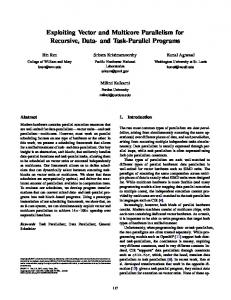
Next, we illustrate in Figure 4 the success of individual rollout policies at reducing delay, and the ability of parallel rollout to combine the effects of rolling out different base policies without knowing ahead of time which base policy is better. The figure compares advantages of the parallel rollout policy in comparison with rollout policies constructed from individual buffer-k policies for various values of k, showing that parallel rollout performs as well as the best of the individual rollout policies, thus achieving the intent of
18
relieving the system designer of a possibly difficult choice. It turns out that for the buffer management problem, rollout of buffer-25 dominates the other individual rollout policies for all traffics and throughput constraints — it remains to be seen how parallel rollout performs when combining base policies that lead to incomparable individual rollout policies, which is the case for the scheduling problem. Traffic 1
Traffic 2
0.018
0.016
0.01
0.009
rollout buffer−25
0.008
rollout buffer−20
0.014
0.007
rollout buffer−25 rollout buffer−20
rollout buffer−13
Average Delay
Average Delay
0.012
0.01
0.008
0.006 rollout buffer−13 0.005
0.004
rollout buffer−7 0.006
0.003 0.004
0.002 rollout buffer−7
0.002
0.001
parallel rollout 0 0
5
10 15 Tolerance %
20
parallel rollout 0 0
25
5
10 15 Tolerance %
20
25
Traffic 4
Traffic 3 0.018
0.025
0.016
0.02
rollout buffer−25 0.014
rollout buffer−25
rollout buffer−20
rollout buffer−20
0.015
Average Delay
Average Delay
0.012
rollout buffer−13
0.01
0.01
rollout buffer−13
0.008
rollout buffer−7 0.006 rollout buffer−7 0.004
0.005
parallel rollout 0.002 parallel rollout
0 0
5
10 15 Tolerance %
20
0 0
25
5
10 15 Tolerance %
20
25
Figure 4: Comparison of parallel rollout of buffer-k policies with individual rollout of various buffer-k policies.
In sum, our results show that rollout provides a sampling-based control approach that can exploit a provided traffic model to improve significantly on simple non-model-based controllers (e.g., RED/buffer-k policies), reducing the queueing delay achievable for a fixed loss constraint by nearly a factor of two when the loss constraint is not extremely tight (little dropping is possible without some risk of loss of throughput). Moreover, our results indicate that our new parallel rollout technique successfully combines simple 19
buffer management policies, relieving the system designer of the need to select which base policy to roll out (a choice that may be traffic dependent). Furthermore, for non-strict loss constraints, we can see that the parallel rollout approach often reduces queueing delay very nearly to the theoretical limit provided by our new offline algorithm given in Appendix C. B. Multiclass Scheduling Problem We first describe three basic online scheduling policies that use no information about the distribution of arrival patterns to provide a baseline for comparison with sampling-based approaches. The first is static priority (SP), which serves the highest-cost class that has a task unscheduled that is live at each time (breaking ties by serving the earlier arriving task). The second is earliest deadline first (EDF) where the policy EDF serves the class with the earliest-expiring task unscheduled that is live at each time (breaking ties by serving the higher class task). The last is current minloss (CM) policy, which first generates the set of the tasks such that serving all of the tasks in the set gives the maximum weighted throughput provided that there is no future task arrivals, and then selects a task in the set such that the CM policy maximizes the unweighted throughput over any finite interval. It has been shown that the CM policy is a good greedy policy over many interesting traffics and is provably no worse than EDF for any traffic. See Givan et al. (2001)’s work for the substantial discussion on this policy. As before, we are faced with the problem of selecting a test traffic. In scheduling, this problem manifests itself in the form of arrival patterns that are easily scheduled for virtually no loss, and arrival patterns that are apparently impossible to schedule without heavy weighted loss (in both cases, it is typical that blindly serving the highest class available performs as well as possible). Difficult scheduling problems are typified by arrival patterns that are “close” to being schedulable with no weighted loss, but that must experience some substantial weighted loss. As before, we have conducted experiments by selecting at random HMM models for the arrival distributions from a guided ad-hoc but reasonable single distribution over HMMs. The study of relationship between HMM models and schedulability would be a good future topic. All of the problems we consider involve seven classes (1 through 7) of tasks. We set the weights of the seven classes such that class i has a weight of wi-1. By decreasing the parameter w in [0,1], we accentuate the disparity in importance between classes, making the scheduling problem more class-sensitive. We show below how performance depends on w. Note that at the one extreme of w=0, SP is optimal, and at the other extreme of w=1, EDF/CM is optimal. We select an HMM for each class, chosen from the same distribution. We selected the HMM state space of size 3 (arbitrarily) for these examples, resulting in a total hidden state space of 37 states. We deliberately arrange the states in a directed cycle to ensure that there is interesting dynamic structure to be modeled by the POMDP information-state update (we do this by setting the non-cyclic transition probabilities to zero). Similarly, we select the self-transition probability for each state uniformly in the interval [0.9, 1.0] in order that state transitions are seldom enough that observations 20
as to what state is active can accumulate. The arrival generation probability at each state is selected such that one state is “low traffic” (uniform in [0, 0.01]), one state is “medium traffic” (uniform in [0.2, 0.5]), and one state is “high traffic” (in [0.7, 1.0]). Finally, after randomly selecting the HMMs for each of the seven classes from the distribution, we used the stationary distribution obtained over the HMM states to normalize the arrival generation probabilities for each class so that arrivals are (roughly) equally likely in high-reward (classes 1 and 2), medium-reward (classes 3 and 4), and low-reward (classes 5–7), and to make a randomly generated traffic from the HMM have overall arrivals at about 1 task per time unit to create a scheduling problem that is suitably saturated to be difficult. Even with these assumptions, a very broad range of arrival pattern HMMs can be generated. Without some assumptions like those we made here, we have found (in a very limited survey) that the arrival characterization given by the HMMs generated is typically too weak to allow any effective inference based on projection into the future. As a result, CM typically performs just as well, and SP often performs nearly as well. Given the selected distribution over HMMs, we have tested the rollout algorithm with CM as the base policy, rollout with SP as the base policy, parallel rollout with CM and SP as base policies (EDF is not used because CM dominates EDF for any traffic), and the CM algorithm, along with SP and EDF, against four different specific HMM arrival descriptions drawn from the distribution. For each such arrival description, we ran each scheduling policy for 62,500 time steps and measured the competitive ratio achieved by each policy. The “competitive ratio” is the ratio between the performance of an online algorithm and the optimal offline performance for the same traffic, which can be obtained from Peha and Tobagi (1990). Here, we use weighted loss as the measure of performance, and compute the optimal offline performance as just described. Examination of the competitive ratio in Figure 5 first reveals that the basic CM policy dramatically outperformed EDF and SP on all the arrival patterns over almost all values of w. For the values of w that are very close to zero, SP starts to dominate CM, which is not surprising owing to the very high accentuation of the disparity among classes. This shows that CM is evidently a good heuristic policy that can be used for the (parallel) rollout algorithm. However, this does not necessarily mean that the rollout algorithm with CM performs well even though we can expect that it will improve CM. Furthermore, it is very difficult to predict in advance the performance that will be achieved by rollout with SP, even though SP is not competing with CM very well. Overall, all sampling-based approaches improved the performance of CM. This is more noticeable in the region of medium to low w values because as we increase the value of w, the performance of CM gets closer to the optimal performance and there is not enough theoretical margin for improvements. It is quite interesting that the rollout of SP performs quite well (even though SP itself is not competing well), which shows that the ranking of Q-values guided by rolling out SP is well-preserved. As we expected, there is a cross point between the rollout of SP and the rollout of CM for each traffic showing that for different class21
Traffic 1
Traffic 2
10
10 EDF
9
9
8
8
EDF
Empirical competitive ratio
Empirical competitive ratio
SP SP
7
6
5
CM
4
7
6
5 CM 4 ROCM
ROCM 3
3 ROSP
2
2
ROSP
PARA PARA 1 0
0.2
0.4
ω
0.6
0.8
1 0
1
0.2
0.4
Traffic 3
0.8
1
0.6
0.8
1
10
9
9
EDF
8
EDF
8
SP
7
Empirical competitive ratio
Empirical competitive ratio
0.6
Traffic 4
10
6
5
4
7
6 SP 5
CM
4
CM
ROCM
ROCM 3
3 ROSP
2
2 PARA
1 0
ω
0.2
ROSP PARA
0.4
ω
0.6
0.8
1 0
1
0.2
0.4
ω
Figure 5: Empirical competitive ratio plots for four different traffics from four different traffic models. ROCM is rollout with CM as the base policy, ROSP is rollout with SP as the base policy, and PARA is parallel rollout with CM and SP as the base policies. For this competitive ratio, the offline optimization solution algorithm by Peha and Tobagi (1990) was used to obtain the theoretical bound.
disparity measures, the performances of the rollout depend on the base policy selected. From the figure, we can see that the parallel rollout policy in comparison with rollout policies constructed from CM and SP policies performs no worse than the best of the individual rollout policies for almost all w values, thus again achieving the intent of relieving the system designer of a possibly difficult choice. For some w values, it even improves both rollout approaches by 10-20% for the rollout of SP and by 10-45% for the rollout of CM. Furthermore, at w no bigger than 0.3, it improved CM about 30-60%, let alone improved SP. In particular at w very near zero, it improved CM and/or SP in one order of magnitude. Note that as the value of w decreases from 1 (but not too close to 0), the complexity of the scheduling problem gets more diffi22
cult. This result is quite expected because SP is the right choice for traffic patterns with heavy bursts of important class packets, whereas CM is the right choice for the other traffic patterns, roughly speaking. Rolling out these policies at the same time makes the resulting parallel rollout approach adapt well to the right traffic pattern automatically. We believe these results advocate our main points for parallel rollout and indicate that sampling to compute the Q-function via parallel rollout is a reasonable heuristic for online scheduling. We expect that it will continue to be difficult to find any distributions where CM outperforms parallel rollout—these would be distributions where the estimated Q-function was actually misleading. It is not surprising that for some HMM distributions, both CM and parallel rollout perform very similarly, as the state inference problem for some HMMs can be very difficult—parallel rollout will perform poorly if the computed information-state represents significant uncertainty about the true state, giving a poor estimate of the future arrivals. VI. CONCLUSION In this paper, we proposed a practically viable new approach, parallel rollout, to solving (partially observable) Markov decision processes via online Monte-Carlo simulation. The approach generalizes the rollout algorithm of Bertsekas and Castanon by rolling out a set of multiple heuristic policies rather than a single policy, and resolves the key issue of selecting which policy to roll out among multiple heuristic policies whose performances cannot be predicted in advance, and improves on each of the base policies by adapting to the different system paths. Our parallel rollout framework also gives a natural way of incorporating given traffic models to solve controlled queueing process problems. It uses the traffic model to predict future arrivals by sampling and incorporates the sampled futures into the control of queueing process. We considered two example controlled queueing process problems, a buffer management problem and a multiclass scheduling problem, showing the effectiveness of parallel rollout. We believe that the applicability of the proposed approach is very wide and in particular, is very effective in the domain of problems where multiple base policies are available such that each policy performs near-optimal for a different set of system paths. In this respect, the approach is quite naturally connected with state-aggregation approach to reduce the complexity of solving various POMDP problems. REFERENCES Anderson, A.T., Jensen, A., and Nielsen, B. F. 1995. Modelling and performance study of packet-traffic with self-similar characteristics over several timescales with Markovian arrival processes (MAP). Proc. 12th Nordic Teletraffic Seminar: 269–283. Anderson, A. T., and Nielsen, B.F. 1997. An application of superpositions of two state Markovian sources to the modelling of self-similar behaviour. Proc. IEEE INFOCOM: 196–204. Asmussen, S., Nerman, O., and Olsson, M. 1996. Fitting phase-type distributions via the EM algorithm. Scand. J. Statist., Vol. 23: 419–414. 23
Bertsekas, D. P. 1995. Dynamic Programming and Optimal Control. Athena Scientific. Bertsekas, D. P. 1997. Differential training of rollout policies. Proc. 35th Allerton Conference on Communication, Control, and Computing, Allerton Park, IL. Bertsekas, D.P., and Castanon, D. A. 1999. Rollout algorithms for stochastic scheduling problems. J. of Heuristics, Vol. 5: 89–108. Bertsekas, D. P., and Tsitsiklis, J. 1996. Neuro-Dynamic Programming, Athena Scientific. Blondia, C. 1993. A discrete-time batch Markovian arrival process as B-ISDN traffic model. Belgian J. of Operations Research, Statistics and Computer Science, Vol. 32. Chang, H.S. 2001. On-line sampling-based control for network queueing problems, Ph.D. thesis, Dept. of Electrical and Computer Engineering, Purdue University, West Lafayette, IN. Chang, H.S., Givan, R., and Chong, E. K. P. 2000. On-line scheduling via sampling. Proc. 5th Int. Conf. on Artificial Intelligence Planning and Scheduling: 62–71. Chen, D. T., and Rieders, M. 1996. Cyclic Markov modulated Poisson processes in traffic characterization. Stochastic Models. Vol. 12, no.4: 585–610. Duffield, N. G. and Whitt, W. 1998. A source traffic model and its transient analysis for network control. Stochastic Models, Vol.14: 51–78. Fischer, W., and Meier-Hellstern, K. 1992. The Markov-modulated Poisson process (MMPP) cookbook. Performance Evaluation, Vol. 18: 149–171. Floyd, S., and Jacobson, V. 1993. Random early detection gateways for congestion avoidance. IEEE/ACM Trans. Net., Vol. 1, no. 4: 397–413. Givan, R., Chong, E. K. P., and Chang, H. S., Scheduling multiclass packet streams to minimize weighted loss, Queueing Systems (QUESTA), to appear. Hashem, E. 1989. Analysis of random drop for gateway congestion control. Tech. Rep. LCS/TR-465, Massachusetts Institute of Technology. Ho, Y. C., and Cao, X. R. 1991. Perturbation Analysis of Discrete Event Dynamic Systems. Norwell, Massachusetts: Kluwer Academic Publishers. Kearns, M., Mansour, Y., and Ng, A. Y. 1999. A sparse sampling algorithm for near-optimal planning in large Markov decision processes. Proc. 16th Int. Joint Conf. on Artificial Intelligence. Kearns, M., Mansour, Y., and Ng, A. Y. 2000. Approximate planning in large POMDPs via reusable trajectories. To appear in Advances in Neural Information Processing Systems 12, S. A. Solla, T. K. Leen, K.-R. Müller, eds., MIT Press. Kitaeve, M. Y., and Rykov, V. V. 1995. Controlled Queueing Systems. CRC press, 1995. Kulkarni, V. G., and Tedijanto, T. E. 1998. Optimal admission control of Markov-modulated batch arrivals to a finite-capacity buffer. Stochastic Models, Vol. 14, no. 1: 95–122. Mayne, D. Q., and Michalska, H. 1990. Receding horizon control of nonlinear system. IEEE Trans. Auto. Contr., Vol. 38, no. 7: 814–824. Misra, V. M.,and Gong, W. B. 1998. A hierarchical model for teletraffic. Proc. IEEE CDC, Vol. 2: 1674– 1679. Neuts, M. F. 1979. A versatile Markovian point process. J. Appl. Prob., Vol. 16: 764–779. Peha, J. M., and Tobagi, F. A. 1990. Evaluating scheduling algorithms for traffic with heterogeneous performance objectives. Proc. IEEE GLOBECOM: 21–27. Puterman, M. L. 1994. Markov Decision Processes: Discrete Stochastic Dynamic Programming. Wiley, New York. Romanov, A. and Floyd, S. 1995. Dynamics of TCP traffic over ATM network. IEEE J. of Select. Areas Commun., Vol. 13, no. 4: 633–641. Ross, S. M. 1997. Simulation. Academic Press. Turin, J. W. 1996. Fitting stochastic automata via the EM algorithm. Stochastic Models, Vol. 12: 405–424.
24
APPENDIX A: Policy Switching Analysis for Total Reward ps We assume that the policy switching policy πps is given by a sequence { µ ps 0 , …, µ H s – 1 } of different
state-action mappings, where each µt is selected by the policy switching method given Equation (8) for horizon Hs–t. π ps
π
Theorem 2: Let Π be a nonempty finite set of policies. For πps defined on Π, V H ( x ) ≥ max π ∈ Π V H ( x )
for all x ∈ X . Proof: To prove the theorem, we will use induction on i, backwards from i = H down to i = 0, showing for π ps
each i that for every state x, V H – i π ps
π
V 0 ( x) = V 0 π ps V H – (i + 1) ( x )
π
( x ) ≥ max π ∈ Π V H – i ( x ) . As the base case, for i = H, we have
( x ) = 0 for all x in X and for any π in Π by definition. Assume for induction that π
≥ max π ∈ Π V H – ( i + 1 ) ( x ) for all x. Consider an arbitrary state x. From standard MDP the-
ory, we have π
π
ps ps V Hps– i ( x ) = E w { r [ x, µps i ( x ), w ] + V H – ( i + 1 ) ( f ( x, µ i ( x ), w ) ) } .
(16)
Using our inductive assumption and then interchanging the expectation and the maximization, Equation (16) becomes: π
π ps V Hps– i ( x ) ≥ E w { r [ x, µps i ( x ), w ] + max π ∈ Π V H – ( i + 1 ) ( f ( x, µ i ( x ), w ) ) }
(17)
π ps
π ps V H – i ( x ) ≥ max π ∈ Π E w { r [ x, µps i ( x ), w ] + V H – ( i + 1 ) ( f ( x, µ i ( x ), w ) ) }.
By definition, µps i ( x ) is the action selected by the policy argmax π ∈ Π Ew{ r [ x, π ( x ), w ] + π
V Hπ – i – 1 ( f ( x, π ( x ), w ) ) }, i.e. by the policy arg max π ∈ Π V H – i ( x ) . It follows that there exists a policy π′ in Π that achieves this argmax; i.e., such that π
π′
E w { r [ x, π′(x), w ] + V H – i – 1 ( f ( x, π′( x), w ) ) } = max π ∈ Π V H – i ( x ) and π′ ( x ) = µps i ( x) .
(18)
Now observe that the definition of “max” implies that π'
E w { r [ x, π′ ( x ), w ] + V H – i – 1 ( f ( x, π′ ( x ), w ) ) } π ps ≤ max π ∈ Π E w { r [ x, µps i ( x ), w ] + V H – i – 1 ( f ( x, µ i ( x ), w ) ) }
Therefore,
π
.
(19) π
π ps V Hps– i ( x ) ≥ max π ∈ Π E w { r [ x, µps i ( x ), w ] + V H – i – 1 ( f ( x, µ i ( x ), w ) ) } ≥ max π ∈ Π V H – i ( x ) ,
which completes the proof. Q.E.D.
APPENDIX B: Parallel Rollout and Policy Switching Analysis for Infinite Horizon Discounted Reward
Here we extend our analytical results for parallel rollout and policy switching to the infinite-horizon discounted-reward case. In this case, we focus only on stationary policies, as there is always an optimal 25
policy that is stationary. Given an initial state x0, we define the expected discounted reward over infinite horizon of a stationary policy π with a discounting factor γ in (0,1) by π
V ( x0 ) = E {
∑∞t = 0 γ r [ xt, π ( xt ), wt ] } where xt+1 is given by f (xt,π(xt),wt) . t
(20)
Note that this definition is an extension of the total expected reward over a finite horizon H we defined earlier by letting H = ∞ and providing a discount factor to ensure convergence to a finite value. We now prove that given a set of base stationary policies, Π = {π1, …, πm}, the expected discounted rewards over infinite horizon of both policy switching and parallel rollout policy on Π are no less than that of any policy in Π. Let V denote the set of functions from X to ℜ (the “value functions”). Define for each π ∈ Π , an operator VIπ: V → V
such that for a value function v ∈ V on each x ∈ X ,
V I π ( v ) ( x ) = r [ x, π ( x ) ] + γ
∑ p ( y x, π ( x ) )v ( y ) where r [ x, π ( x ) ]
y∈X
= E w ( r [ x, π ( x ), w ] ) .
(21)
From the standard MDP theory, it is well known that VIπ is a contraction mapping in a complete normed linear space, or Banach space, that there exists a unique fixed point v ∈ V satisfying VIπ(v) = v, that this fixed point is equal to Vπ, and that iterative VIπ on any initial value function converges monotonically to this fixed point. We first state a key lemma, which will be used to prove our claim. π
Lemma: Suppose there exists ψ ∈ V for which V I π ( ψ ) ( x ) ≥ ψ ( x ) for all x ∈ X , then V ( x ) ≥ ψ ( x ) for all x ∈ X . The above lemma can be easily proven by the monotonicity property of the operator VIπ and the convergence to the unique fixed point of Vπ from successive applications of the operator. We can now state and prove our infinite horizon results. Theorem 3: Let Π be a nonempty finite set of stationary policies. For πps defined on Π,
V
π ps
π
( x ) ≥ max π ∈ Π V ( x ) for all x ∈ X . π
Proof: Define ψ ( x ) = max π ∈ Π V ( x ) for all x ∈ X . We show that V I πps ( ψ ) ( x ) ≥ ψ ( x ) for all x ∈ X , and then by the above lemma the result follows. Pick an arbitrary x. By definition, π
π'
π
π ps ( x ) = ( arg max π V ( x ) ) ( x ) . Therefore, there exists a policy π' ∈ Π such that V ( x ) ≥ V ( x ) for all π ∈ Π and π ps ( x ) = π' ( x ) . It follows that VI πps ( ψ ) ( x ) = r [ x, π ps ( x ) ] + γ = r [ x, π' ( x ) ] + γ
∑ p ( y x, πps ( x ) )ψ ( y )
y∈X
∑ p ( y x, π' ( x ) )ψ ( y )
y∈X
≥ r [ x, π' ( x ) ] + γ
∑ p ( y x, π' ( x ) )V
y∈X π'
= V ( x ) = ψ ( x ). 26
π'
( y)
(22)
By the lemma above, the claim is proved. Q.E.D. Theorem 4: Let Π be a nonempty finite set of stationary policies. For πpr defined on Π,
V
π pr
π
( x ) ≥ max π ∈ Π V ( x ) for all x ∈ X . π
Proof: Define ψ ( x ) = max π ∈ Π V ( x ) for all x ∈ X . We show that V I πpr ( ψ ) ( x ) ≥ ψ ( x ) for all x ∈ X so that the result follows by the lemma above. Fix an arbitrary state x. By definition, π pr ( x ) = arg max u ∈ U ( x ) r [ x, u ] + γ p ( y x, u )ψ ( y ) . Then, for any π ∈ Π ,
∑
y∈X
VI πpr ( ψ ) ( x ) = r [ x, π pr ( x ) ] + γ ≥ r [ x, π ( x ) ] + γ
∑ p ( y x, πpr ( x ) )ψ ( y )
y∈X
∑ p ( y x, π ( x ) )ψ ( y )
y∈X
≥ r [ x, π ( x ) ] + γ
∑ p ( y x, π ( x ) )V
π
by def. of π pr and def. of argmax (23)
( y ) by def. of ψ
y∈X π
= V ( x ). π
Therefore, V I πpr ( ψ ) ( x ) ≥ max π ∈ Π V ( x ) = ψ ( x ) . By the lemma above, the claim is proved. Q.E.D.
APPENDIX C: Offline Buffer Management
For the buffer management problem, the offline performance analysis corresponds to finding the optimal dropping plan for any given traffic arrival sequence (with respect to the objective function given in Section IV.B in formalizing buffer management). In this section we give a novel characterization of the optimal dropping plan, provide a new algorithm for computing this optimal plan, and prove the correctness and claimed time complexity for that algorithm. A. Defining and Characterizing the Optimal Plan Throughout this section, we focus on a fixed arrival sequence at, t ∈ {0, .., Hs–1}, where Hs is our sampling horizon, and discuss how to find an optimal dropping plan for that sequence. All the definitions below are relative to this fixed arrival sequence. We begin by formally defining the problem. A dropping plan is a sequence of nonnegative integers d = [d0, d1, …, d H s – 1 ] giving the number of packets dt to drop at each time t. We refer to the empty dropping plan [0, …, 0] as φ. Given a dropping plan d, the unbounded queue-length trajectory lt(d) under that plan is given by the following evolutionary equations: l0 ( d ) = a0 – d 0 l i + 1 ( d ) = min ( 0, l i ( d ) – 1 ) + a i + 1 – d i + 1
(24)
Note that there is no limit on buffer size incorporated here. The plan d is said to meet buffer constraint k if 27
lt(d) is does not exceed k for any t. The cumulative reward associated with a dropping plan is given by Hs – 1
R(d) =
∑ sgn ( l (d) ) – λ ( l (d) ) , t
t
(25)
t=0
and we say that a dropping plan is optimal if it meets buffer constraint N and achieves cumulative reward on the given arrival sequence at no less than any other plan meeting constraint N. We now define an optimal plan δ and prove its optimality. The intuition behind this plan is that our reward function R(d) is such that we prefer to drop any packet that must wait 1/λ time steps for service. It follows that we must do just enough dropping to ensure no packet must wait 1/λ time steps — moreover, we must drop any packet that will be dropped (either for the reason just given or for buffer overflow) the moment it arrives, in order to minimize queue length. Likewise, we must avoid dropping any packet when an earlier-arriving packet has yet to be served; instead, dropping the earlier arriving packet. We now formalize these ideas. Given a dropping plan d, the next empty time at time t, denoted n(d, t), is the least time t’ ≥ t such that l t’ ≤ 1. This is the first time not before t at which the queue will be empty after service if we follow plan d, ignoring the limit on buffer size. We say that a dropping plan d is acceptable at time t if the next empty time at time t, n(d, t) is less than min(t + (1/λ), Hs–1), and the queue trajectory l t’ (d) is less than or equal to the buffer size N for all times t’ in the interval [t, n(d, t)]. We note that acceptability is monotone relative to increased dropping: if d is acceptable at time t, than any plan d’ that drops no less than d at each time step is also acceptable at t. Also, this definition ensures that an acceptable trajectory leaves the queue empty at the horizon, after the last service interval. In the definition below, we treat a partial dropping plan [d0, ..., dt] for some t ≤ H s as a full dropping plan by assuming that dt’ is zero for all t’ in the interval (t,Hs]. Note that under this interpretation, [] is the empty dropping plan (drops no packets). Definition 1: The dropping plan δ = [ δ 0, …, δ H s – 1 ] is defined recursively as follows: for all i ≥ 0, δi = the smallest x such that the time i is acceptable relative to the dropping plan [δ0, ..., δi–1, x]. We now establish that the plan δ is an optimal dropping plan. Theorem 5: δ is an optimal dropping plan for the fixed arrival sequence used to define it.
Proof: It is not difficult to show that each of the following “helpful” local transformations on a dropping plan d = [d0, d1, …, d H s – 1 ] results in a dropping plan d’ = [d’0 , d’1 , …, d’H s – 1 ] that is no worse than d. Here, “no worse” means that the sequence yields at least as much cumulative reward. • [Helpful Transformation 1] The sequence d’ agrees with d at all times except that at one time t we have d’t = dt – 1 and d’ is acceptable at t. 28
• [Helpful Transformation 2] The sequence d’ agrees with d at all times except that at one time t, we have d’t = dt + 1 and d is not acceptable at t. • [Helpful Transformation 3] The sequence d’ agrees with d at all times except two times t and t’ such that t < t’, d’t = dt + 1, d’t’ = dt’ – 1, where d and d’ are acceptable at both t and t’, and n(d,t) ≥ t’. (This transformation can be applied whenever there is a drop called for in the presence of earlier-arriving packets in order to drop those instead.) Using these transformations, we can argue that the following fact holds: (*) For any i in the interval [0, Hs–2], for any dropping sequence d such that dt = δt for all t in the interval [0, i], there exists a dropping sequence d’ such that d’t = δ t for all t in the interval [0, i+1] and d’ is no worse than d. The optimality of δ then follows by induction because the fact (*) just shown implies that given any plan we can find one no worse that follows δ initially for more time steps. Applying this fact at most Hs times shows that δ is no worse than any arbitrary plan. Q.E.D. B. A Method for Computing the Optimal plan In Figure 7 we give pseudocode for an O(Hs log Hs) algorithm for computing the plan δ described in the previous subsection (δ is called plan[] in the pseudocode), and we explain the design of this code here. The algorithm assumes we have already computed the unbounded queue-length trajectory lt ([]) for no dropping and stored the trajectory in traj[t], for each t — this is easy to do in O(Hs) time. The main loop of the algorithm scans this trajectory using a time-valued index variable looktime. A second time index variable droptime also moves through the time interval [0, Hs) in a monotonically increasing fashion, marking the location in plan[] that is currently being updated. As droptime is increased, the variable offset is maintained to summarize the relevant effect of the dropping actions selected for time indices 0 through droptime–1 — specifically, the difference between the no-dropping trajectory lt ([]) and the trajectory under the dropping policy given by the current plan[], where the difference computed applies at any time t between droptime and the next empty time under plan[], which is no earlier than looktime. The variable droptime does not have to take on every value in [0, Hs–1] due to the following property. Given dropping action δi from the plan δ, the definitions of acceptability and of the plan δ imply that the actions δj for all j in the interval (i, m] for m = n([δ0, …, δi], i) are all zero. This fact justifies updating droptime to the next empty time plus one after each dropping action is selected. During the looktime scan (i.e., in the body of the main for loop), the following computations are performed to select dropping actions. Whenever looktime encounters an overflow, or reaches a point at least 1/ λ steps ahead of droptime without finding the next empty time, it is necessary to add to the amount of dropping done at droptime in order to make plan[] acceptable at droptime. The amount of dropping added is
29
int plan[Hs]; /* storage for result, init to zero everywhere */ int traj[Hs]; /* init traj[t] to unbounded queue size lt([]) */ droptime = offset = 0; for looktime = 0 to Hs–1 do if ( traj[looktime] – offset == 0 ) then /* lt[plan[]] is 0 for t=looktime so offset decreases and no further dropping until after looktime */ if ( offset > 0 ) then offset = offset – 1; endif droptime = looktime + 1; else /* check/resolve if droptime arrivals wait too long */ if ( looktime ≥ droptime + 1/λ) then mintime = argmin{t ∈ [droptime,looktime]} traj[t]; dropamt = traj[mintime] – offset – 1; plan[droptime] = plan[droptime] + dropamt; offset = offset + dropamt; droptime = mintime + 1; endif /* check/resolve any buffer overflow at looktime */ if (looktime == Hs–1) then bufsize=1; else bufsize = N; endif excess = traj[looktime] – offset – bufsize; while ( excess > 0 ) do mintime = argmin{t ∈ [droptime,looktime]} traj[t]; dropamt = min{excess, traj[mintime] – offset – 1}; plan[droptime] = plan[droptime] + dropamt; excess = excess – dropamt; offset = offset + dropamt; /* if lmintime(plan[]) ≤ 1 then no further dropping until after mintime */ if ( traj[mintime] – offset == 1 ) then droptime = mintime + 1; endif endwhile if ( traj[looktime] – offset == 1) then droptime = looktime + 1; endif endif endfor Figure 7: Pseudocode for an offline optimizing algorithm for buffer management. The argmin lines must break ties to prefer later times.
selected (in the lines using “argmin” and “min” to set dropamt) to ensure that either the buffer overflow is prevented, or that a queue-empty time occurs between droptime and looktime (the latter is required if looktime is at 1/λ steps ahead of droptime). If the amount of dropping added results in an empty queue between droptime and looktime, then droptime is advanced to one more than this empty time. Likewise, if the looktime scan encounters a point at which the trajectory is empty under plan[], then droptime is advanced beyond this point. 30
The operation “argmin” is used in the pseudocode shown in two places, in each case to select the minimum amount of dropping to add to the plan at time droptime in order to cause the next empty time under the resulting plan to be earlier than looktime. This use of “argmin” ensures that we drop only the minimum number of packets at droptime to either avoid buffer overflow at looktime or ensure a next empty time before looktime. Specifically, “argmin” is used to compute the lowest point in the unbounded droppingfree trajectory between droptime and looktime (breaking ties in favor of the latest time) — it follows that dropping (at droptime) all but one packet in the current trajectory at that time is the least additional drop at droptime that results in an empty time in the interval [droptime, looktime]. We then drop that amount if an empty time is sought (i.e., after the first use of “argmin” in the pseudocode) or possibly less than that amount if we are only seeking to avoid buffer overflow (i.e., after the second use of “argmin”). A final point worth remarking on is the handling of the queue at the horizon. Because the optimal dropping sequence must leave the queue empty after the last service (in order that all unserved packets are dropped as early as possible), we must have the line of code that sets bufsize to 1 when looktime reaches the horizon. This line, together with the final if statement updating droptime ensure that droptime equals Hs on termination, and that the resulting plan leaves the buffer empty at time Hs. We next discuss the correctness of the code shown. C. Correctness and Time Complexity We argue below that the pseudocode shown in Figure 7 actually computes the desired plan δ, and does so in O(Hs log Hs) time. Note that once we find the optimal plan, computing R(d) as needed for hindsight optimization is straightforward. Theorem 6: The code in Fig. 7 computes the plan δ.
Proof: The following invariants can be proven together by induction to hold of the code in Fig. 7. • The variables offset and droptime are maintained so that the variable offset takes the value lt([]) – lt(plan) on each entry to the for loop body, for any t in the interval [droptime, looktime] (the difference does not depend on t in this interval). • The variable droptime is always less than or equal to looktime on entry to the for loop body. • plan[t] = δ t for all t < droptime. • plan[t] = 0 for all t > droptime. • plan[t] ≤ δ t for t = droptime. • traj[droptime]–offset > 1 on entry to the main if statement, unless droptime = looktime. • On entry to the for loop, the unbounded queue-length trajectory for the dropping specified in plan[] shows neither buffer overload nor a queue of size 0 or 1 in the time interval [droptime, looktime). • The variable looktime is never greater than droptime+1/λ when the for loop is entered. 31
These invariants, together with the easily proven fact that droptime = Hs on termination establish that plan[t] = δt for all t when the algorithm terminates. Q.E.D. We now discuss the time complexity of the algorithm. Theorem 7: The code in Fig. 7 runs in O(Hs log Hs) time.
Proof: The two argmin operations can be supported by a priority queue implemented as a heap in O(log Hs) time per invocation. The number of iterations of the main loop is clearly Hs. Each operation in the body of this loop, excluding the while loop, takes at most log(Hs) time, so the amount of time spent in the main for loop altogether (excluding the inner while loop) is O(Hs log Hs). To conclude, we must argue that the total time spent in the while loop is at most O(Hs log Hs). We first observe that the while loop body takes at most log Hs time for a single iteration, and then argue that over the entire algorithm at most Hs iterations occur. We divide such iterations into two groups: terminal iterations and continuing iterations, where a “terminal iteration” is one after which the while loop terminates, and a “continuing iteration” is followed by yet another iteration of the loop. We note that there can be at most O(Hs) terminal iterations of the while loop because such iterations are followed inevitably by the end of an iteration of the for loop. But it is easy to show that continuing iterations occur only when dropamt = traj[mintime] – offset – 1 (i.e., dropamt is less than excess due to the min{...} application), and that droptime is increased at every such iteration. It is also possible to show that droptime starts at 0, never decreases, and is never greater than Hs. Therefore there can be at most O(Hs) increases in droptime and as a result at most O(Hs) continuing iterations. We conclude that the while loop iterates at most O(Hs) times. Q.E.D.
32