Numerical Linear Algebra with Applications 4: 43{66. CSW96]Chapman A., Saad Y., and Wigton L. (1996) High-order ILU preconditioners for CFD problems.
51
Parallel Solution of General Sparse Linear Systems using PSPARSLIB 1
2
Yousef Saad , Sergey Kuznetsov , Gen-Ching Lo
3
Distributed Sparse Linear Systems PSPARSLIB [SM95] is a portable package for solving sparse linear systems on parallel platforms. The package adapts a number of methods based on domain decomposition concepts to general sparse irregularly structured linear systems. It is implemented in FORTRAN 77 with a few C functions and uses the MPI communication library for message passing. This paper describes some of the methods implemented in the package and examines a number of strategies used to improve their performance. Given a large sparse nonsymmetric real matrix A of size n, we consider the linear system Ax = b; (1) that can arise, for example, from a nite element discretization of a partial di�erential equation. To solve this system on a distributed memory computer, it is common to partition the nite element mesh and assign a cluster of elements representing a physical subdomain to each processor. Each processor assembles only the local equations associated with the elements assigned to it. When the system is already in 1 University of Minnesota, Department of Computer Science and Engineering, Minneapolis, MN. Work supported in part by ARPA under grant NIST 60NANB2D1272 and in part by NSF under grant CCR-9618827. Additional computational resources were provided by the Minnesota Supercomputer Institute and by the University of Minnesota IBM Shared Project. 2 Institute of Mathematics, Novosibirsk, Russia. This work was carried out while the author was on leave at the University of Minnesota, Department of Computer Science and Engineering, Minneapolis, MN. 3 Morgan-Stanley, New-York Eleventh International Conference on Domain Decomposition Methods Editors Choi-Hong Lai, Petter E. Bj�rstad, Mark Cross and Olof B. Widlund c 1999 DDM.org
PSPARSLIB
465
(a) (b)
External interface points Internal points
External data
O
Local Interface points
Figure 1
local Data
Ai
Xi
External data
O Xi
A local view of a distributed sparse matrix.
assembled form, subsets of equations-unknowns are assigned to processors. In either case, each processor will wind up with a set of equations (rows of the linear system) and a vector of the variables associated with these rows. A distributed linear system is a set of linear equations that are assigned in this fashion to a distributed memory computer. This paper presents the general principles used in a parallel iterative sparse linear system solver with an emphasis on de ning preconditioners for distributed sparse linear systems. These (global) linear systems of equations are regarded as distributed objects and solution methods must be developed by exploiting the local data structures associated with the distributed linear system. The rst step of any parallel sparse iterative solver is to set up these local data structures. In this preprocessing phase, the local equations are represented along with the dependencies between the local variables and external variables, and any other information needed during the iteration phase. We will give a brief overview of the local representation of the linear system and discuss how the solution package is built around this representation. A number of variations of some known preconditioning techniques will then be presented. The Local System.
Figure 1-(a) shows a `physical domain'viewpoint of a sparse linear system which is akin to that used in the domain decomposition literature. A point (node) in a `subdomain' is actually a pair representing an equation along with an associated unknown. It is common to distinguish between three types of unknowns: (1) Interior variables which are coupled only with local variables by the equations; (2) Local interface variables which are those coupled with non-local (external) variables as well as local variables; and (3) External interface variables which are variables in other processors that are coupled with local variables. We can also represent the related local equations as shown in Figure 1-(b). Note that these equations are not contiguous in the original system. The matrix represented in the gure can be viewed as a reordered version of the equations associated with a local numbering of the equations/unknowns pairs. As can be seen in Figure 1-(b), the rows of the matrix assigned to a certain processor have been split into two parts: a local matrix A which acts on the local variables and an interface matrix X which acts on remote variables. These remote variables must i
i
466
SAAD, KUZNETSOV, AND LO
be received from other processor(s) each time that a matrix-vector product with the matrix A is performed. It is common to list the interface nodes last, after the interior nodes. This local ordering of the data leads to e�cient interprocessor communication, and reduces local indirect addressing during matrix-vector products. The zero blocks shown are due to the fact that local internal nodes are not coupled with external nodes. Each local vector of unknowns x consists of the subvector u of internal nodes followed by the subvector y of local interface variables. The right-hand side b is conformally split into the subvectors f and g , and the local matrix A residing in processor i as de ned above is block-partitioned according to this splitting. The local equations can therefore be written as follows. � �� � � � � � B E u + P 0 = fg (2) F C E y y 2 The block matrix on the left side is the local matrix A . Here, N is the set of subdomains that are neighbors to subdomain i. Each term E y in the sum in the left-hand side is the contribution to the local equation from neighboring subdomain number j. The subvectors of external interface variables are grouped into one vector called y and the notation X E y �Xy i
i
i
i
i
i
i
i
i
i
i
i
i
i
j
Ni
ij
j
i
i
i
ij
j
i;ext
j
ij
2
j
i
i;ext
Ni
will be used to denote the contributions from external variables to the local system (2). In e�ect, this represents a local ordering of the external variables. With this notation, the left-hand side of (2) becomes w = A x +X y (3) The vector w is the local part the matrix-by vector product Ax in which x is a vector which has the local vector components x , i = 1; : : :; s. To facilitate matrix operations and communication, an important task is to gather the data structure representing the local part of the linear matrix as was just described. In this preprocessing phase it is also important to form any additional data structures required to prepare for the intensive communication that will take place during the solution phase. In particular, each processor needs to know (1) the processors with which it must communicate, (2) the list of interface points and (3) a break-up of this list into pieces of data that must be sent and received to/from the \neighboring processors". A complete description of the data structure associated with this boundary information is given in [SM95] along with additional implementation details. i
i
i
i
i;ext
i
i
Matrix-vector operations.
The matrix-vector product is carried out according to equation (3). First, the external data y needed in each processor is obtained. The matrix-vector product with the matrix A on the local data x can be carried out at the same time that this communication step is being performed. Then the matrix-vector product with the i;ext
i
i
PSPARSLIB
467
matrix X on the external data y can be carried out and the result is added to the result obtained from A x . The following is a code segment for performing this operation as it is implemented in PSPARSLIB. i
i;ext
i
c c c c c
i
send local interface data to neighbors call MSG_bdx_send(nloc,x,y,nproc,proc,ix,ipr,ptrn,ierr) do local matrix-vector product for local points call amux(nloc,x,y,aloc,jaloc,ialoc) receive remote interface date from neihgbors call MSG_bdx_receive(nloc,x,y,nproc,proc,ix,ipr,ptrn,ierr) peform matrix-vector product with external data and add it to current result vector y nrow = nloc - nbnd + 1 call amux1(nrow,x,y(nbnd),aloc,jaloc,ialoc(nloc+1)) return
Here MSG send and MSG receive are subroutines that invoke the proper MPI calls for sending and receiving the interface data to and from neighboring processors. The send is non-blocking. The set of parameters nproc, proc, ix, ipr, ptrn, contains precisely the data structure needed for the interface variables.
Distributed Krylov Subspace Solvers The main operations in a standard Krylov subspace acceleration are (1) vector updates, (2) dot-products, (3) matrix-vector products and (4) preconditioning operations. If we exclude the matrix-vector products (discussed above) and preconditioning steps (to be seen later), the rest of the operations in an algorithm such as CG or GMRES are mainly dot-products and vector updates. Since vector quantities are split in the same fashion, a global SAXPY of two vectors across p processors, consists of p independent SAXPYs. In contrast, a global dot product requires a global sum of the separate dot products of the subvectors in each processor. The dot products are mainly used in orthogonalizing sets of Krylov vectors and this constitutes one of the potential bottlenecks in a parallel implementation of Krylov subspace procedures. Experience shows however, that in most practical situations the loss of e�ciency due to inner products is usually minor unless the sub-problems become relatively small[KLS97]. One of the main Krylov accelerator used in PSPARSLIB is the exible variant of GMRES [SS86] known as FGMRES [Saa93]. This is a right-preconditioned variant that allows the preconditioning to vary at each step. Since the preconditioning operations require solving systems associated with entire subdomains it becomes important to allow the preconditioner itself to be an iterative solver. This means that the GMRES iteration should allow the preconditioner to vary from step to step within the inner GMRES process. A variant of GMRES which allows this is called the exible variant of GMRES (FGMRES), see [Saa93] for details. It is important to implement the accelerators (e.g. FGMRES) with \reverse communication", a mechanism whose goal is to avoid passing data structures to the accelerator. When calling a standard FORTRAN subroutine implementation of an
468
SAAD, KUZNETSOV, AND LO
. . D1 .. D2 D3 .. D4 : : : S1 : : : : : : S 2 : : : . . D5 .. D6 D7 .. D8 An example of splitting eight domains on the plane into two groups
Table 1
iterative solver, we normally need to pass a list of arguments related to the matrix A and to the preconditioner. This can be a burden on the programmer because of the rich variety of existing data structures. The solution is not to pass the matrices in any form. When a matrix { vector product or a preconditioning operation is needed, the subroutine exits and the calling routine performs the desired operation and then calls the subroutine again, after placing the desired result in one of the vector arguments of the subroutine. For details, see [SW95, Saa95, Saa96]. Variants of Additive Schwarz Preconditioners.
The additive Schwarz procedure is a form of block Jacobi iteration, in which the blocks refer to systems associated with entire domains. Each iteration of the process consists of the following steps: (1) Obtain external data y ; (2) Compute (update) local residual r = (b ? Ax) = b ? A x ? X y (3) Solve A � = r ; and (4) Update solution x = x + � . To solve the systems in step 3, a standard (sequential) ILUT preconditioner [Saa96] combined with GMRES or one step of an ILU preconditioner is used. Of particular interest in this context are the overlapping additive Schwarz methods. In the domain decomposition literature, see e.g., [Bj�89, BW89, SBG96] among others it is known that overlapping is a good strategy to reduce the number of steps. There are however several di�erent ways of implementing overlapping block Jacobi iterations, for example, we can replace the data in the overlapping subregions by its external version or use some average of the data. It is sometimes possible to reduce the number of outer iterations required by block Jacobi preconditioners by using a 2-level clustering of the subdomains. The subdomains are split into groups S1 ; S2 ; : : :; S . The assignment of the subdomains to groups can be determined from knowledge of neighboring subdomains. Figure 1 shows an example in which 8 subdomains are split into two groups. Consider a certain group of subdomains, say S , and the set of equations-unknowns corresponding to all the subdomains belonging to S . The local system for subdomain i 2 S can be rewritten in the form: A x + Z z + (X y ? Z z ) = w where z is a part of the vector y corresponding to remote variables in the same group as subdomain i, Z is a part of the interface matrix X which acts on the remote variables z . Thus the solution of the linear system A x +Z z = w will provide a preconditioner for the (outer) block Jacobi iteration. This nested twolevel form of the block Jacobi iteration, can be described as follows. i;ext
i
i
i
i
i
i
i
i
i;ext
i
i
i
i
p
k
k
i
i
k
i
i;ext
i;ext
i
i;ext
i
i;ext
i
i;ext
i
i
i;ext
i
i
i
i;ext
i
PSPARSLIB
469
Algorithm 1 Hierarchical Block Jacobi Iteration 1. Obtain external data y 2. Compute (update) local residual r = (b ? Ax) = b ? A x ? X y 3. Do i = 1; : : :; i1 4. Obtain external data z 5. Compute (update) local residual s = r ? Z z 6. Solve A � = s 7. End 8. Update solution x = x + � i;ext
i
i
i
i
i
i
i;ext
i;ext
i
i i
i
i
i
i;ext
i
i
i
The number of inner iteration i1 depends on the problem. Often, the choice i1 = 2 achieves a good compromise between accuracy for the local block solver and overall performance. The hierarchical block Jacobi iteration presents several advantages over the traditional block Jacobi iteration. It allows to reduce the number of outer iterations due to increased accuracy in the preconditioning step. On the other hand, this approach increases communication costs which can be reduced by using small groups. Variants of Multiplicative Schwarz Preconditioners.
The multiplicative Schwarz preconditioner uses the same extended domains as the additive Schwarz method, but the subdomain solves are sequential: every processor uses interface variables de ned by preceding local solves. The simplest form of the multiplicative Schwarz is the block Gauss-Seidel algorithm used in domain decomposition techniques [BW86, SBG96, CM94]. A partial remedy to the sequential nature of the multiplicative Schwarz technique is to use multi-coloring. Thus, if the domains are colored, the multiplicative Schwarz as executed in each processor would involve a color loop through all the colors - and execution of the loop is performed only when the color variable equals the color of the processor, see [SBG96, Saa96]. The rest of the iteration is identical with that of Additive Schwarz. A problem with multicoloring is that as the domain associated with the given color is active, all other colors will be inactive. As a result it is typical to obtain only 1=numcol e�ciency where numcol is the number of colors. To reduce this e�ect, one can further block the local variables into two blocks: interior and interface variables. Then the global SOR iteration is performed with this additional blocking. In e�ect, each local matrix A is split as � � � � � � B 0 + 0 E = (4) A = FB E F 0 0 C C where the B part corresponds to internal nodes. The resulting segregated multiplicative Schwarz is as follows, Algorithm 2 Segregated multiplicative Schwarz 1. Solve B � = r 2. x := x + � 3. Do col = 1 ; : : :; numcols 4. If (col :eq :mycol ) then i
i
i
i
i
i
i;x
i;x
i;x
i
i
i
i
i
i
i
i
470
5. 6. 7. 8. 9.
SAAD, KUZNETSOV, AND LO
Obtain external data y Update y-part of residual r Solve C � = r Update interface unknowns y = y + � EndIf The advantage of this procedure is that the bulk of the computational work in each domain is done in parallel. Loss of parallelism comes from the color loop which involves only solves with interface variables, which are of lower complexity. i;ext
i;y
i i;y
i;y
i
i
i;y
Numerical Experiments In this section, we report on some results obtained when solving distributed sparse linear systems on an IBM SP2 with 14 nodes, an IBM cluster of 8 workstations, and an SGI Challenge cluster and a 64 processor CRAY-T3E. The SGI challenge workstation cluster consists of three 4-processor Challenge L servers and one 8processor Challenge XL server. The processors on the Challenge L and XL are the same (R10,000) but the memory sizes are di�erent. Communication between di�erent SGI cluster workstations (respectively, IBM RS/6000 workstations) can be performed via a HiPPI (High Performance Parallel Interface) switch or a Fibre-Channel switch. On the IBM cluster, an ATM switch is used. The MPI communication library is used for all communication calls. The ATM and HiPPI are high speed interfaces and can transfer data at 155 Mbps and 800 Mbps, respectively. The IBM RS/6000 Model 590 workstations are based on the Power2 architecture. The SP2 nodes communicate with an internal switch which achieves a bandwidth of 320 Mbps bandwidth and has a latency of about 40 microseconds. The CRAY-T3E has 64 nodes and 128 Megabytes of memory per node. The processors are connected in a 3-D torus by a network capable of 480 Mbps in each direction for each link.
Experiments with block Jacobi preconditioning. First, we compare the three di�erent overlapping options mentioned at the end of Section 51, when they are used in conjunction with the block Jacobi iteration using. The results are summarized in Figure 2. In the gures, jacno stands for block Jacobi with no overlapping, jaco av for block Jacobi with overlapping and averaging of the overlapping data, jac for block Jacobi with overlapping and exchange of overlapped data. A standard ILUT preconditioner combined with GMRES was used as a local solver and the number of inner iterations was equal to its = 11. We select its = 11 because it minimizes the execution time for a small number of processors if preconditioned GMRES is used as a local solver. Note that the optimal set of parameters depends on the number of processors and the problem considered. It is sometimes reasonable to use a smaller number for the level of ll or a smaller number of inner iterations if the number of processors is large. The results are for the matrix VENKAT01 of dimension 62,424 with 1,717,792 non-zero entries on the CRAY-T3E, using a relative tolerance of " = 10?6, a Krylov subspace dimension of m = 50 and a ll-in of 25 for the ILUT preconditioner. The comparison shows that overlapping can reduce the number of outer iterations and jac usually requires fewer iterations.
PSPARSLIB
471
Jacobi overlapping . Matrix VENKAT01. CRAY−T3E 18 16
time in seconds
14 12
_______jac
10
.........jacno −−*−−−−jac_av
8 6 4 2 0 0
5
10 15 Number of processors
20
25
20
25
Matrix VENKAT01. CRAY−T3E 20
Number of outer iterations
19
18
17
16 __________jacno 15
................jac −−*−−−*−−−jac_av
14
13 0
5
10 15 Number of processors
Figure 2 Comparison of FGMRES with distributed block Jacobi preconditioner for three di�erent overlapping strategies on the CRAY-T3E. Left plot: execution times. Right plot: Iterations
472
SAAD, KUZNETSOV, AND LO
Number of processors preconditioned GMRES ILU solver
1 3 5 10 time 16.34 9.64 5.59 2.96 speed-up 1.69 2.92 5.52 its 13 16 17 18 time 8.85 3.78 2.49 1.39 speed-up 2.34 3.55 6.37 its 15 18 20 21
16 24 2.35 1.66 6.95 9.84 19 19 1.04 0.77 8.51 11.49 21 21
Execution times in seconds, speed-up and number of outer iterations for the block Jacobi preconditioner with two di�erent local solvers
Table 2
PEs Matvecs Seconds Table 3
8 10 16 20 399 493 589 727 308.21 254.38 170.85 165.66
Number of matrix-vector multiplications and execution times (seconds) for the BARTH1S matrix.
The ILUT factorization is often more economical. Table 2 gives timing results, speedups and iteration counts for the block Jacobi preconditioner with overlapping using two di�erent local solvers. Table its shows the number of FGMRES steps. These results are given for the VENKAT01 matrix on the CRAY-T3E, using a relative tolerance of " = 10?6 , a Krylov subspace dimension of m = 50 and a level of ll of 25 for the ILUT preconditioner. These tests and others, indicate that using ILUT as a local solver (without any acceleration) is faster than using preconditioned GMRES preconditioned with ILUT. Several approaches can be used to improve the load balance among processors. One approach is to adapt the number of inner iterations for each processor based on the time consumed by the preconditioning step for a few rst iterations. Numerical tests on the SP2 and on the IBM RS6000 show that this `forced load balancing' approach can yield a 10% to 25 % reduction in the execution time when the number of processors is small, see [KLS97] for details. The next matrix, referred to as BARTH1S, was supplied by T. Barth of NASA Ames, see [CSW96]. It models a 2D high Reynolds number airfoil problem, with turbulence. The matrix has a 5x5 block structure and has 189,370 rows and 6,260,236 nonzero entries. This linear system is very ill-conditioned (see [CSW96]) and very hard to solve iteratively. We had to use a de ated version of GMRES [CS97]. The local systems are solved using one step of an ILU solve, where the LU factors are obtained from a block ILU(k) preconditioner (see [CSW96]) where k denotes a level of ll. Table 3 gives the timing results, and the number of matrix-vector multiplications. The following parameters have been used: the level of ll was 4, the number of de ated eigenvectors was 8, the Krylov subspace dimension was 50, and the tolerance threshold was 1.E-5.
PSPARSLIB
473 Method its = 1 its = 2 its = 3 its = 5 ILU sol Matvecs 238 108 127 106 238 Seconds 15.23 9.88 15.08 18.02 15.147
Table 4
Performance of the hierarchical Jacobi preconditioner with di�erent number of inner steps and for the ILU solve.
Experiments with hierarchical block Jacobi. We now compare the overlapping
Jacobi preconditioner with the forward-backward LU solver and the hierarchical Jacobi preconditioner for 2-D elliptic problems. It is assumed that all processors have been split into groups by means of the following function f (j) de ned by: f (j) = b(j ? 1)=bc + 1, where b is a blocking factor for processors. Table 4 shows performance results for the hierarchical block Jacobi preconditioner using four di�erent numbers of inner iterations. The results are for a Poisson equation on the unit square. The number of processors is 8, the problem size is 90,000. A standard forwardbackward local ILU solver was used. The blocking factor for processors is 2, the tolerance is 10?6, the level of ll is 5, and the Krylov subspace dimension is 30. b
b
An increase in the number of inner iterations leads to a signi cant reduction in the number of outer iterations. However, the execution time increases as the number of inner iterations increases from 2 to 5 due to higher computational costs of each step. The number of inner iterations of 2 seems to give the best compromise in this case.
Experiments with Multiplicative Schwarz. Figure 3 shows a comparison of multiplicative Schwarz for four di�erent types of local solution strategies on the CRAYT3E for the VENKAT01 matrix. As was already explained, the Multicolor SOR scheme used here involves substantial idle time for each processor since only one color is active at any given time. It is therefore much less e�cient than the other methods. The gure shows once again that requiring more accuracy for the ILU local solves leads to a reduction in the total time. Also the use of a single ILU solve leads to good savings in computational time.
REFERENCES [Bj�89] Bj�rstad P. E. (1989) Multiplicative and Additive Schwarz Methods: Convergence in the 2 domain case. In Chan T., Glowinski R., P�eriaux J., and Widlund O. (eds) Domain Decomposition Methods. SIAM, Philadelphia, PA. [BW86] Bj�rstad P. E. and Widlund O. B. (1986) Iterative methods for the solution of elliptic problems on regions partitioned into substructures. SIAM Journal on Numerical Analysis 23(6): 1093{1120. [BW89] Bj�rstad P. E. and Widlund O. B. (1989) To overlap or not to overlap: A note on a domain decomposition method for elliptic problems. SIAM Journal on Scienti c and Statistical Computing 10(5): 1053{1061.
474
SAAD, KUZNETSOV, AND LO Multicolor SOR preconditioning. Matrix VENKAT01. 25
− − o − − multicolor segregated SOR, ILU solver and GMRES 20
− − x − − multicolor SOR with ILU solver .................. multicolor segregated SOR, ILU solver
time in seconds
______________ multicolor SOR 15
10
5
0 0
Figure 3
2
4
6 8 10 Number of processors
12
14
16
Comparison of 4 di�erent multiplicative Schwarz algorithms.
[CM94] Chan T. F. and Mathew T. P. (1994) Domain decomposition algorithms. Acta Numerica pages 61{143. [CS97] Chapman A. and Saad Y. (1997) De ated and augmented Krylov subspace techniques. Numerical Linear Algebra with Applications 4: 43{66. [CSW96] Chapman A., Saad Y., and Wigton L. (1996) High-order ILU preconditioners for CFD problems. Technical Report UMSI 96/14, Minnesota Supercomputer Institute. [KLS97] Kuznetsov S., Lo G. C., and Saad Y. (1997) Parallel solution of general sparse linear systems. Technical Report UMSI 97/98, Minnesota Supercomputer Institute, University of Minnesota, Minneapolis, MN. [Saa93] Saad Y. (1993) A exible inner-outer preconditioned GMRES algorithm. SIAM Journal on Scienti c and Statistical Computing 14: 461{469. [Saa95] Saad Y. (1995) Krylov subspace methods in distributed computing environments. In Hafez M. (ed) State of the Art in CFD, pages 741{755. [Saa96] Saad Y. (1996) Iterative Methods for Sparse Linear Systems. PWS publishing, New York. [SBG96] Smith B., Bj�rstad P., and Gropp W. (1996) Domain decomposition: Parallel multilevel methods for elliptic partial di�erential equations. Cambridge University Press, New-York, NY. [SM95] Saad Y. and Malevsky A. (1995) PSPARSLIB: A portable library of distributed memory sparse iterative solvers. In et al. V. E. M. (ed) Proceedings of Parallel Computing Technologies (PaCT-95), 3-rd international conference, St. Petersburg, Russia, Sept. 1995. [SS86] Saad Y. and Schultz M. H. (1986) GMRES: a generalized minimal residual algorithm for solving nonsymmetric linear systems. SIAM Journal on Scienti c and Statistical Computing 7: 856{869. [SW95] Saad Y. and Wu K. (1995) Design of an iterative solution module for a parallel sparse matrix library (P SPARSLIB). In Schonauer W. (ed)
PSPARSLIB Proceedings of IMACS conference, Georgia, 1994.
475