Parallel Direct Solution of Linear Equations on FPGA-Based Machines* Xiaofang Wang and Sotirios G. Ziavras Department of Electrical and Computer Engineering New Jersey Institute of Technology Newark, New Jersey 07102, USA Email:
[email protected]
Abstract The efficient solution of large systems of linear equations represented by sparse matrices appears in many tasks. LU factorization followed by backward and forward substitutions is widely used for this purpose. Parallel implementations of this computation-intensive process are limited primarily to supercomputers. New generations of Field-Programmable Gate Array (FPGA) technologies enable the implementation of System-On-aProgrammable-Chip (SOPC) computing platforms that provide many opportunities for configurable computing. We present here the design and implementation of a parallel machine for LU factorization on an SOPC board, using multiple instances of a soft processor. A highly parallel Block -Diagonal-Bordered (BDB) algorithm for LU factorization is mapped to our multiprocessor. Our results prove the viability of our FPGA-based approach.
Keywords: FPGA, LU factorization, forward/backward substitution, parallel processing, SOPC.
1. Introduction Many scientific and engineering problems, such as circuit simulation, applications in electric power networks and structural analysis, involve solving a large sparse system of simultaneous linear equations. LU factorization is a very efficient and commonly employed direct method to solve such problems. It has been proved in [1] that LU factorization is much faster than non-stationary iterative methods in electric power flow applications that use the Newton-Raphson (NR) method for systems with up to 685 buses. With LU factorization, the solution of the entire system is obtained by solving two sets of triangular equations. However, LU factorization is a computationintensive method, especially for large matrices with ----------* This work was supported in part by the U.S. Department of Energy under grant ER63384.
thousands of elements that frequently appear in these application areas. The motivation to reduce the execution time, especially when operations have to be carried out in real time, has stimulated extensive research in applying parallel processing to the LU factorization of linear systems. Many successful parallel LU solvers have been developed for massively-parallel supercomputers [2, 4, 7]. Although parallel computers have accomplished a great deal of success in solving computation-intensive problems, their high price, the long design and development cycles, the difficulty in programming them, as well as the high cost of maintaining them limit their versatility. For example the scarcity and high cost of parallel architectures available to the industry limits greatly the further application of parallel processing in power engineering [4]. On the other hand, with constant advances in VLSI technologies and architecture design, FPGAs have grown into multi-million-gate SOPC computing platforms, from originally serving as simple platforms for small ASIC prototyping and glue logic implementation. New generations of FPGAs have made it possible to integrate a large number of computation resources, such as logic blocks, embedded memory, fast routing matrices, and microprocessors on one silicon die. It is possible now to build Multi-Processor-On-a-Programmable -Chip (MPOPC) systems, which offer a great opportunity to reevaluate previous research efforts through the employment of the promising configurable computing paradigm. MPOPC designs offer alternative ways to optimize the system and reduce communication overheads that have been long obstacles to parallel processing implementations. The research motivation in this paper is to develop a cost-effective, high-performance parallel architecture for electric power applications based on a new generation of FPGAs. Our shared-memory MIMD multiprocessor machine uses six Altera Nios® configurable IP (Intellectual Property) processors as computation and control nodes and is implemented on the Altera SOPC development board, which is populated with an
1
EP20K1500EBC652-1x FPGA. We have adapted a very efficient parallel sparse matrix solver, namely the Bordered-Diagonal-Block (BDB) solver for sparse linear equations [2]. Our low-cost, high-performance approach can improve the performance of various real-time electrical power system applications, such as power flow and transient stability analysis. It is also applicable to other scientific areas that require the solution of such equations in reasonable running times.
2. Parallel Sparse Bordered-Diagonal-Block Solution 2.1. Introduction to LU Factorization Many problems require the solution to the following set of simultaneous linear equations: Ax = b
(1)
where A is an N x N nonsingular sparse matrix, x is a vector of N unknowns, and b is a given vector of length N. The solvers for this equation come mainly in two forms: direct [5] and iterative [1]. One of the classic direct methods is LU factorization, which works as follows. We first factorize A so that A=LU, where L is a lower triangular matrix and U is an upper triangular matrix. Once L and U are determined, then the equations can be written as two triangular systems, Ly = b and Ux = y, whose solutions can be obtained by forward reduction and backward substitution, respectively. There are many implementations of LU factorization. The "Doolittle LU factorization algorithm” [5] assumes that L has all 1's on the diagonal and can be formulated as: j −1
Lij = ( A ij − Uij = Aij −
∑L
ik * Ukj )*
k =1 i −1
∑L
1 Ujj
for j
∈ [1, i-1]
(2)
for j
∈ [i, N]
(3)
ik * Ukj
k =1
From these equations, we can observe that the Doolittle method can benefit from storing the matrix in the row order for fast matrix accesses. Since our matrices are stored in the row order, we employ the Doolittle method for those parts of our LU factorization that require the application of conventional LU factorization. Compared to iterative algorithms having convergence rates greatly depending on the characteristics of the matrices, LU factorization is more robust because every nonsingular matrix can be factored into some form of two triangular matrices. Also, the result of LU factorization can be used repeatedly after the right hand vector has changed, as is the case for decoupled power flow analysis.
2.2. Parallelization of LU Factorization of Sparse Matrices Many research efforts have targeted parallel LU factorization algorithms for supercomputers and clusters of PCs or workstations [1, 2, 4, 8]. There are several critical issues that a parallel implementation of LU factorization has to address. The most important factor is data dependences. From equations (2) and (3), the calculation of the kth row and column elements requires the solved data on preceding rows and columns. If the matrix elements are distributed to the processors of a parallel computer, then frequent communication among the processors is required, which reduces the efficiency of parallel algorithms and also increases the hardware complexity of custom-made parallel machines. Communication overhead has been a major problem in existing parallel LU factorization algorithms [1,5,7,8]. Another main issue for parallel LU factorization is pivoting. To maintain numerical stability during factorization, pivoting is usually applied by rearranging the rows or/and columns of A at every step in order to choose the largest element as the pivot. Pivoting is more complex in parallel implementations because the permutation of rows or/and columns requires communication and synchronization between processors that greatly increase the complexity of parallel sparse LU factorization. Furthermore, pivoting may cause load imbalance among processors. This problem is further exacerbated if dynamic data structures are employed to store sparse matrices. In SuperLU, static symbolic LU factorization is performed in order to determine in advance all possible fill-ins (positions of zeros in the original matrix that will be replaced with non-zero elements during LU factorization), before actual LU factorization takes place [2, 3]. Fortunately, some applications, such as electric power systems, employ symmetric positive definite matrices which are also diagonally dominant, so pivoting is not often required. Since we do not consider here pivoting during LU factorization, we can use static data structures where the location of all fill-ins is predetermined. In our implementation of parallel LU factorization that targets electric power matrices, we focus on another important purpose of ordering, i.e., to exploit the inherent parallelism in sparse matrices. By using the node tearing technique [6], which will be discussed later, we reorder the nodal admittance matrix of the power network into the Bordered-Diagonal-Block (BDB) form (see the A matrix in Figure 1). The above three major difficulties for parallelization, i.e. data dependences, pivoting and fill-ins, can be attacked efficiently in this form. It was also demonstrated elsewhere that electric power matrices with a maximum value of N equal to a few thousand can be ordered into this form and a related parallel
2
implementation on the Connection Machine CM-5 supercomputer resulted in impressive speedups for up to 16 processors [2].
A11 0 0 A22 ... ... 0 0 An 1 An 2 #1
#2
...
0
... ...
0 ...
... A n − 1 n − 1 ... A nn − 1 # n -1
Processor
A1 n X1 B1 # 1 A2 n X 2 B 2 # 2 ... × ... = ... A n − 1 n X n − 1 Bn − 1 # n-1 A nn X n B n # n-1
# n-1
Figure 1. Sparse BDB matrix In Figure 1, the Aij ’s are matrix blocks; the Aii ’s are referred to as diagonal blocks, and Ain and Anj are called right border blocks and bottom border blocks, respectively, where i,j ∈ [1, n]. The blocks Aii , Ain, and Ani are said to form a 3 -block group, where i∈ [1, n-1] and n ≤ N. Every 3-block group is also associated with a block in the X vector and a block in the right side B vector. The factorization and solution of the 3-block groups can be carried out independently, in parallel. The factorization and solution of the last diagonal block Ann requires data produced in the right and bottom border blocks, so this task is the last step. In order to facilitate the computation in the last block, pairs of border blocks after LU factorization are multiplied together in parallel by every processor to produce S nj=Lnj Ujn, for j ∈ [1, n-1]. Then, the summation is accumulated by all the processors and sent to the processor which is assigned the last diagonal block. Because all other off-diagonal blocks contain all 0’s, there will be no fill-ins outside of these blocks (Aij) during factorization and the result will have the same BDB structure. Moreover, communication is only required in the procedure of accumulating partial sums. Thus, the BDB matrix algorithm exhibits distinct advantages for parallel implementation.
2.3. Parallel Solution for BDB Sparse Matrices Based on the above discussion, we can now form the parallel BDB algorithm for sparse linear systems. We assume a shared-memory MIMD multiprocessor (details follow in Section 4). First we order the A matrix into the BDB form by using the node tearing algorithm introduced in [6]. Node tearing is a very efficient heuristics-based partitioning technique first introduced in the 70s in order to solve large-scale circuit simulation problems. Given a large-scale circuit/network, this technique tries to identify independent groups of nodes and isolate the set of edges running between these independent groups. Thus, the
circuit is divided into sub-circuits that can be dealt with independently, in parallel. After all the equations have been solved for the sub-circuits, we can solve the coupled equations. In our case, the nodes in the graph-circuit represent rows of our symmetric matrix, whereas an edge connecting nodes i and j implies that a non-zero element exists at the intersection of row i and column j. In Figure 1, the independent diagonal blocks correspond to independent sub-networks, and the last (lower right) diagonal and border blocks represent the coupling between the independent sub-networks. Because the last block is factorized in the last step using solution data produced for preceding blocks in the matrix, we should try to make the last block as small as possible (that is, we should try to minimize the number of coupled equations). For large matrices, we may make the number of independent 3-block groups a multiple of the number of processors in the parallel system in order to assign every processor several 3-block groups in the parallel implementation. A large size for the last diagonal block will reduce the performance of the parallel algorithm. Thus, there is an optimal ordering for a given system. For electric power distribution networks the buses are usually loosely interconnected, thus the node tearing algorithm can produce very good results because of the sparsity in the corresponding matrix. Table 1 shows the results of the node tearing algorithm for the admittance matrix of the IEEE 118-bus test system assuming five processors. Table 1. Size of sub-blocks assigned according to node tearing for the IEEE 118-bus system and five processors Case 1
Case 2
Case 3
6
11
16
Processor 1*
23
8,12
6,7,7
Processor 2*
24
8,12
4,7,7
Processor 3*
22
10,10
5,7,7
Processor 4*
20
10,12
6,6,6
Processor 5*
20
10,10
4,7,7
Size of Last Block
9
16
25
L*
L*: Total number of 3-block groups Processor 1-6: Dimensionality of the diagonal blocks assigned to the processor
In Case 1, every processor is assigned one 3-block group. In Cases 2 and 3, we order the matrix in such a way that every processor has two and three 3-block groups, respectively. The size of the last block is much
3
larger in Cases 2 and 3. We compare the performance of the implementation for these different cases in Section 5. We also tried explicit load balancing in the reordering phase. A good load balancing technique should take into account not only the number of equations assigned to each processor but also the actual number of resulting operations from non-zero elements. Minimum degree ordering is applied inside the matrix blocks to get a near optimal BDB matrix in order to reduce the fill-ins and the number of computations. BDB matrices are normally unchanged for non-trivial amounts of time since they represent generators of electricity and existing power distribution networks. Therefore, the extra time consumed in the matrix reordering phase is easily justifiable. After we get the BDB form of the targeted sparse matrix, we can then carry out parallel LU factorization (see Figure 1) as follows. (1) Factorization of the independent 3-block groups in parallel. (2) Multiplication in parallel of the right and bottom border factored blocks within individual processors to generate the partial block sums. (3) Accumulation of these partial results involving processor pairs. (4) Factorization of the last diagonal block using the result of the last step. Thus, every processor originally contains all of the data that it needs to operate on, except for the last block. Only local communications are required in this algorithm. Because the factorization of the last block is a sequential task, the most efficient algorithm is chosen to factor the last block. The factored LU matrix produced by this algorithm is in the BDB format. Thus, it demonstrates inherent parallelism in the forward reduction and backward substitution phases. In forward reduction, the following equation is used: i −1
yi =bi -
∑ (l
ij
* yj )
for i=1, …, N
(4)
j =1
where lij stands for Lij . If the matrix blocks are distributed among the processors in an increasing processor-address row-number order, communication is required to transfer the results in the y vector to the processor with the next higher address before the latter begins its work. However, except for the diagonal blocks in the sparse BDB matrix, all matrix blocks in L used in equation (3) contain all zeros (see Figure 1) so no communication is required between processors. Therefore, solving for the values in the y vector corresponding to the independent diagonal blocks can be carried out in parallel, except for the last block that requires all the solved data of L and the values in the y vector from all processors with lower addresses. We let every processor generate the partial sums after it finds the unknowns in y, which are then accumulated for the last processor by employing a binary tree of processors configuration. The procedure is as follows. (1) All processors operate in parallel to solve the part of the y vector assigned to them, using their assigned diagonal
blocks in matrix L and vector B. (2) All processors perform matrix-by-vector operations in parallel involving their lower border block and the corresponding solved block in the y vector. (3) Partial results are accumulated in parallel by all processors so they can be used in the next step to obtain the solutions in the last diagonal block. (4) Forward reduction is carried out in the last diagonal block by the processor with the highest address. The equation for backward substitution is
x i = yi −
N
∑ (u * x ) ij
j
for i=N, …, 1
(5)
j = i+ 1
where u ij stands for Uij . In our BDB parallel algorithm, we start backward substitution in the last block involving the processor with the highest address. After the solutions are obtained for the last block, this processor broadcasts its solved block for x to all other processors. Finally, all the processors find the solutions in parallel for their assigned block in the x vector.
3. Configurable Computing Configurable or adaptive computing, which is based on the unique advantage of the static and/or run time (re)configurability of FPGA-like or switching devices, has been an intensive research and experimentation area ever since the introduction of commercial FPGAs [9-11]. After more than a decade of exploration, FPGA -based configurable systems can be used as specialized coprocessors, processor-attached functional units or independent processing machines [9], attached message routers in parallel machines, general-purpose processors for unconventional designs [13], and general-purpose or specialized systems for parallel processing [11]. They are able to greatly increase the performance of computationintensive algorithms in DSP, data communication, genetics, image processing, pattern recognition, etc. [9,10]. During recent years, FPGAs have seen impressive improvements in density, speed and architecture. State of the art silicon manufacturing technology not only allows to build faster FPGA chips consisting of tens of millions of system gates, but also allows more features and capabilities with reprogrammable technology. What is interesting is that System-On-a-Chip (SoC) designers are incorporating programmable logic cores provided by FPGA vendors, which can be customized to imp lement digital circuit after fabrication. By using programmable logic cores, ASIC designers can reduce significantly design risks and time. Our research focuses on another advantage of FPGA based configurable systems. FPGAs allow the implementation of various designs in reasonable times. Our designs emphasize hardware parallelism. Currently,
4
the majority of configurable parallel-machine implementations reside on multi-FPGA systems interconnected via a specific network; ASIC components may also be present. For example, Splash 2 uses 17 Xilinx XC4010s arranged in a linear array and also interconnected via a 16 x 16 crossbar [11]. These machines also display substantial communication and I/O problems, like supercomputers. We present here our pioneering experience with the design and implementation of a parallel machine on an SOPC development board for the implementation of parallel LU factorization using the BDB sparse matrix algorithm. Scalability of the algorithm-machine pair is a major objective for high performance (e.g., in power flow analysis). With advances predicted by Moore’s Law, our dependence on SOPC designs will become even more preeminent.
4. Design and Implementation 4.1. Nios Processor and Floating -Point Unit In order to reduce the design and development times, our implementation of a NUMA (Non-Uniform Memory Access) shared-memory multiprocessor employs a commercially available soft IP processor from Altera, namely Nios. The Nios RISC processor is a fully configurable soft IP that offers over 125MHz in the Stratix FPGA. The CPU word size (16-bit or 32-bit), clock speed, register file, SDK, address space, on-chip memory (RAM or ROM), availability of hardware/software multiplier and various other on-chip peripherals can all be tailored to user specifications. In our design, a typical 32-bit Nios takes about 1500 logic elements, which is about 2.9 percent of the logic elements contained in the 1500,000-gate EP20K1500E on the Altera SOPC development board that is used in our implementation. As discussed earlier, the communication overhead has always been a bottleneck for current parallel architectures. So the communication network between processors and peripherals in an IP-based multiprocessor design is a critical element for good system performance. The Nios processors and other peripherals in our parallel machine are interconnected via the fully parameterized and multi-mastering Altera Avalon bus. Unlike the traditional shared bus, it is a fully connected bus, supports simultaneous transactions for all bus masters, and implements arbitration for the slaves (such as on-chip and off-chip memories). LU factorization requires floating-point arithmetic to deal with large dynamic data ranges. Standard Nios instructions support only integer arithmetic operations, but Nios provides an approach that allows the user to significantly increase system performance by
implementing user-defined performance-critical operations through direct hardware instruction decoding. In the past, floating-point units (FPUs) have been rarely introduced in FPGA -based configurable machines due to the space required for FPU implementation; very limited numbers of resources were available in older FPGAs, so designers would choose fixed-point arithmetic in order to leave most of the logic resources to the application implementation. Nowadays, the availability of highercapacity FPGAs makes it more feasible to implement FPUs on FPGAs because of increased numbers of resources [12]. Although many applications based on floating-point arithmetic, especially matrix multiplication, have been implemented in new FPGAs during the last few years, there are still very few reports about configurable systems that have successfully incorporated FPUs. The design and optimization of a very good synthesizable FPU has proved to be a very difficult task. A single-precision (32-bit) IEEE 754 standard FPU was implemented in our project using VHDL; it was ported to a Nios-based system using four user custom instructions. Table 2 shows the performance of our FPU. Table 3 shows that by using a hardwired FPU we can greatly improve the performance of algorithms. Better, commercial IP FPUs are also available but may cost more than $10,000. Table 2. FPU performance for the APEX20K FPGA Functions Adder/ Subtractor Multiplier Divider
System Frequency 51MHz 40MHz 39MHz
Logic Elements 696 2630 1028
Clock Cycles 7 5 50
4.2. Sequential LU Factorization In order to test the performance of the Nios soft IP core and produce comparison data for our parallel solution on the SOPC, sequential LU factorization was first implemented for a single 32-bit Nios containing 128 registers and an FPU; the Altera Nios development board, which is equipped with a EP20K200EFC484-2x FPGA, was used. This Nios processor takes about 5900 logic elements and the maximum system frequency is 40MHz. Table 4 shows the execution times of LU factorization for various matrix sizes and the electric power IEEE 118-bus test system. We can see that for such computationintensive algorithms, the hardware implementation of the FPU results in much faster implementations. The FPGA on the Nios board can only host one processor with a FPU. So we target our multiprocessor design to a highercapacity Altera board, the SOPC development board.
4.3. Multiprocessor Implementation on the SOPC
5
We designed and implemented a parallel Nios-based configurable, MIMD machine on the SOPC board, containing five computation Nios processors and one control Nios processor. Compared to the Nios development board, the SOPC board is almost a "blank" board to us. We first carefully designed the CPU systems according to the requirements of our parallel BDB algorithm. The configurability of the Nios processor offers many ways to customize our system to get good performance. The FPGA device on the SOPC development board, the EP20K1500EBC652-1x, has 51,840 logic elements and 442,368 bits of on-chip memory. In our system, every Nios is a 32-bit processor without hardware multipliers (we use the FPU instead), and contains 128 registers, 7KB on-chip RAM, and 1KB on-chip ROM. Every Nios is coupled with an FPU. The control processor communicates with the host via an onchip UART interface. We also had to develop all the interfaces for most components on the SOPC board, such as the SSRAM, UART, LCD, LED, and buttons, and implemented them as standard SOPC builder library components according to the specifications of the Altera Avalon bus. We do not use any operating system with our parallel machine and the communication between the processors is implemented via on-chip memory. The control program stored in the on-chip ROM of each Nios guides the processor. The monitor program of Nios 6 is used to control and debug the entire system. Whenever the power is turned on or the system is reset, the embedded control program prepares each processor for execution of the application program. In order to save space in the on-chip memory, we coded the boot programs for all the processors in the Nios assembly language and stored them in a 1KB on-chip ROM. The SOPC board provides more than 50KB of on-chip memory and each Nios CPU uses about 1KB for its register file (with the choice of 128 registers), so we assigned every Nios 7KB of on-chip RAM. All Nios processors use the on-board SSRAM as the program memory. The two SSRAM chips on the SOPC have separate address and data buses, and control signal channels. This architecture improves the system frequency and increases memory throughput. Otherwise, with six Nios simultaneously accessing the same SSRAM chip, the SSRAM arbitration would slowdown significantly the system’s operation. We assigned three Nios systems the SSRAM 1 with address range 0x100000~0x1FFFFF and the other two Nios systems the SSRAM 2 with the address range 0x200000~0x2FFFFF. Nios 6 can access both SSRAMs in order to control the system and send the results to the host. We divided the SSRAM memory space into segments and assigned the same amount of memory to each Nios for the main program and data storage. The SRAM chips on the SOPC
board are synchronous, burst SRAMs (SSRAMs). Unlike the zero-wait -state asynchronous SRAM on the Nios board for which all operations take one cycle, normally there are two wait states for a read operation. In our experimentation, we first compared the performance of our programs on the Nios and SOPC boards for only one Nios. Table 5 shows that LU factorization takes about 70 percent more time to run on the SOPC board than on the Nios board due to the larger SSRAM access latency on the SOPC board. In order to reduce the commu nication overhead and take advantage of the fully connectivity of the Avalon bus, the partial block results for the factorization of the last diagonal block and the two substitutions are accumulated in pairs: (1) Nios 1 + Nios 2 -> Nios 2; Nios 3 +Nios 4 -> Nios 4. (2) Nios 2 + Nios 5 -> Nios 5. (3) Nios 4 + Nios 5 ->Nios 5. The complexity of our parallel N BDB algorithm for sparse matrices is O( ( ) 3 ), where p p is the number of processors (the proof is omitted here for the sake of brevity).
5. Performance Results We first tested our parallel BDB LU factorization algorithm, which is expected to dominate the total execution time for solving the linear equations, for different matrix sizes (see Table 6). Here the number of independent diagonal blocks is the same as the number of computation processors (i.e., 5). We observed that, when the size of the blocks assigned to the processors is a power of two, then each Nios works more efficiently. Higher efficiency then may be the result of smoother pipelined accesses of matrix data in the memory. This table shows that the speed-ups are significant for the parallel implementation, which proves the viability of our FPGA -based approach in solving such problems efficiently and at low cost. Table 7 shows the execution times for the forward and backward substitution with these matrices. We can see that with increases in the matrix size, the time spent on LU factorization becomes a more significant component of the total time, which is not surprising provided that LU factorization time increases N as O( ( ) 3 ) while substitution times increase as p
N 2 ) ), where p is the number of processors p participating in the computation. We also compared the performance for different matrix orderings as shown in Table 1 for the IEEE 118-bus test system. Table 8 shows the execution times of LU factorization and substitutions for the three cases in Table 1. For LU factorization, we can see that Case 2 takes less O( (
6
time than the other two cases and Case 3 results in the slowest implementation. Case 2 produces the best performance despite the fact that it imposes significant communication and synchronization overheads because it reduces much faster the computation times in the individual sub-blocks. In contrast, in Case 3 the reduction in computation times for the sub-blocks does not compensate for the significant increases in the former overheads. For the forward and backward substitution, however, the division into sub-blocks has not any effect at all from an individual processor's point of view; in fact, this subdivision increases some overheads in the code for this task. But since LU factorization time dominates the total solution time, an optimal ordering set is still preferable in order to reduce the total solution time. The optimal set may vary with different architectures because the computation-communication ratio may vary. The reordering is performed on the PC host and all the execution times do not include the time corresponding to reordering.
6. Conclusions This paper presents our pioneering experience with the design and implementation of a shared-memory multiprocessor computer on an FPGA -based SOPC board. A parallel BDB algorithm for the solution of linear systems of equations was tested on this parallel system and good performance was obtained. By using a node tearing technique, large sparse matrices can be reordered into the BDB form and LU factorization and forward and backward substitution can be carried out efficiently in parallel. A uni-processor design was also implemented in order to compare the performance with our parallel implementation. The results demonstrate that there exists a best ordering for a given matrix on the targeted machine based on various computation-communication ratios. Our results prove that the new generation of FPGA -based SOPCs provides viable platforms for implementing highperformance parallel machines.
[1] R. Bacher and E. Bullinger, "Application of Non-stationary Iiterative Methods to an Exact Newton-Raphson Solution Process for Power Flow Equations," Proc. 12th PSCC Power Systems Computations Conf., Aug. 1996, pp. 453459. [2] D.P. Koester, S. Ranka, and G.C. Fox, “Parallel BlockDiagonal-Bordered Sparse Linear Solvers for Electrical Power System Applications, ”IEEE Proc. Scal. Paral. Lib. Conf., 1994, pp.195-203. [3] J.J. Grainger and W.D. Stevenson, Jr., Power System Analysis, McGraw Hill Publ., 1994. [4] D.J. Tylavsky, et al. “Parallel Processing in Power Systems Computation,” IEEE Trans. Power Systems, Vol. 7, No 2, May 1992, pp. 629-638. [5] I. S. Duff, A. M. Erisman, and J. K. Reid, Direct Methods for Sparse Matrices, Oxford Univ. Press, Oxford, 1990. [6] A. Sangiovanni-Vincentelli, L. K. Chen, and L. O. Chua, "Node-Tearing Nodal Analysis," Techn. Rep. ERL-M582, Electronics Research Laboratory, University of California, Berkeley, October 1976. [7] C. Fu, X. Jiao, and T. Yang, “Efficient Sparse LU Factorization with Partial Pivoting on Distributed Memory Architectures,” IEEE Trans. Paral. Distr. Systems, Vol. 9 Issue 2, Feb.1998, pp. 109-125. [8] T. Feng and A.J. Flueck, “A Message-Passing DistributedMemory Parallel Power Flow Algorithm,” IEEE Power Engin. Soc. Winter Meet., Vol. 1, 2002, pp. 211 –216. [9] K. Compton, S. Hauck, “Reconfigurable Computing: A Survey of Systems and Software,” ACM Comp. Surv., Vol. 34, Issue 2, June 2002, pp. 171-210. [10] R. Tessier and W. Burleson, “Reconfigurable Computing and Digital Signal Processing: A Survey,” J. VLSI Signal Proc., May/June 2001, pp. 8-27. [11] D. A. Buell, J. M. Arnold, and W. J. Kleinfelder, Splash 2: FPGAs in a Custom Computing Machine, IEEE Computer Society Press, Los Alamitos, CA, 1996. [12] W. Ligon, S. McMillan, G. Monn, K. Schoonover, F. Stivers, and K. Underwood. "A Re-Evaluation of the Practicality of Floating-Point Operation of FPGAs," Proc. FCCM, 1998, pp. 206–215. [13] S. Ingersoll and S.G. Ziavras, “Dataflow Computation with Intelligent Memories Emulated on Field-Programmable Gate Arrays (FPGAs)," Microproc. Microsys., Vol. 26, No. 6, Aug. 2002, pp. 263-280.
. References Table 3. Execution time (in clock cycles) for software and hardware floating-point operations with Nios Operations Addition/Subtraction Multiplication Division
Software (SW) Library Macros 770 2976 1137
Hardware (HW) FPU* 19 16 51
Speedup 40.5 186.0 22.3
* Total time for Nios to complete the entire instruction, including fetching and decoding
7
Table 4. Uni-processor execution time (msec) for LU factorization and substitutions on the Altera Nios development board LU with SW FP
Matrix Size 24 x 24 36 x 36 64 x 64 96 x 96 102 x 102 IEEE 118-bus system
LU with HW FPU
Speedup
99.85845 344.69124 2115.08535 6840.39006 8248.38399
610701 1902411 9978486 32806368 39228519
13643.063514
602.34276
16.35 18.12 21.20 20.85 21.03 22.65
Table 5. Uni-processor execution time (in clock cycles) for LU factorization on the Nios and SOPC boards Programs SW FP
Nios board HW FPU
SOPC board SW FP HW FPU
Multiplication of two floating-point numbers 5x5 LU factorization
2976
16
4376
33
45,168
4583
78,785
7664
30x30 LU factorization
7,570,660
351,843
13,592,766
674,385
Table 6. Execution time (msec) for parallel LU factorization Matrix Size Total Time (msec) Multiprocessor
24x24 0.551
30x30 1.218
36x36 0.957
42x42 1.390
48x48 2.673
54x54 4.438
96x96 15.61
Uni-processor Speedup
1.991 3.61
4.129 3.39
3.400 3.55
5.072 3.65
10.372 3.88
16.793 3.78
62.778 4.02
102x102 21.30 85.10 3.995
Table 7. Parallel execution time (msec) for forward reduction and backward substitution on the SOPC Matrix Size Time (msec) Matrix Sparsity (% of non-zero elements) Forward
24x24
30x30
36x36
42x42
48x48
54x54
96x96
102x102
28.5
25.8
27.5
29.4
25.5
22.2
21.3
23.9
0.060
0.090
0.099
0.124
0.152
0.210
0.475
0.683
Backward Total Time (msec)
0.073 0.133
0.099 0.189
0.115 0.214
0.146 0.270
0.178 0.330
0.238 0.448
0.573 1.048
0.584 1.267
Table 8. Parallel solution times (msec) for the IEEE 118-bus test system on the SOPC
LU factorization Forward
Case 1 15.315 0.497
Case 2 14.030 0.637
Case 3 17.131 0.880
Backward
0.581
0.642
0.882
Total Time
16.393
15.309
18.893
8