Parallel Strategies for an Inverse Docking Method Romain Vasseur
Stéphanie Baud
†‡
[email protected]
Xavier Vigouroux ‡
Laurent Martiny †
[email protected]
[email protected]
†
†
[email protected]
Luiz Angelo Steffenel
[email protected]
Michaël Krajecki
[email protected]
Manuel Dauchez
†
[email protected]
Multi-scale Molecular Modeling Platform (P3M), University of Reims Champagne-Ardenne, France UMR CNRS 6237 MEDyC, SiRMa Laboratory, University of Reims Champagne-Ardenne, France SYSCOM Team, CReSTIC Laboratory, University of Reims Champagne-Ardenne, France ‡ BULL SAS, Education & Research, Echirolles, France
ABSTRACT Molecular docking is a widely used computational technique that allows studying structure-based interactions complexes between biological objects at the molecular scale. The purpose of the current work is to develop a set of tools that allows performing inverse docking, i.e., to test at a large scale a chemical ligand on a large dataset of proteins, which has several applications on the field of drug research. We developed different strategies to parallelize/distribute the docking procedure, as a way to efficiently exploit the computational performance of multi-core and multi-machine (cluster) environments. The experiments conducted to compare these different strategies encourage the search for decomposing strategies as a way to improve the execution of inverse docking.
Categories and Subject Descriptors C.2.4 [Distributed Systems]: Client/Server; Distributed Applications. J.2 [Physical Sciences and Engineering]: Chemistry. J.3 [Life and Medical Sciences]: Biology and genetics.
General Terms Measurement, Performance, Design, Experimentation.
Keywords Molecular docking, inverse docking, blind docking, masterworker, task stealing
1. INTRODUCTION Molecular docking is a widely used computational technique that allows studying structure-based interactions complexes between biological objects at the molecular scale. Molecular docking includes several kinds of studies according to the type of objects involved in the complex: some of the most known are protein-
Permission to make digital or hard copies of all or part of this work for personal or classroom use is granted without fee provided that copies are not made or distributed for profit or commercial advantage and that copies bear this notice and the full citation on the first page. Copyrights for components of this work owned by others than the author(s) must be honored. Abstracting with credit is permitted. To copy otherwise, or republish, to post on servers or to redistribute to lists, requires prior specific permission and/or a fee. EuroMPI '13, September 15 - 18 2013, Madrid, Spain Copyright is held by the owner/author(s). Publication rights licensed to ACM. ACM 978-1-4503-1903-4/13/09…$15.00. http://dx.doi.org/10.1145/2488551.2488584
ligand complex, protein-protein complex, nucleic acids-protein complex and protein-carbohydrates complex. In the field of drug discovery or drug design, molecular docking is focused on protein-ligand complexes to study how the chemical ligand that is a medicine will bind the target protein receptor. The prediction of the binding mode of a ligand into a protein target cavity, the structure of the interaction complex and the estimation of the binding affinity between both is essential to build new therapeutic compounds to fight against life threatening diseases. Molecular docking represents a virtual alternative to costly and time-consuming systematic wet biological experiments as high or medium throughput screening processes (HTS) and NMR-based screens. Then, it is called virtual HTS (vHTS), virtual or in silico ligand screening (VLS) and has become a method of choice for rational drug design, hits identification and hits to leads optimization to complement existing methods [1][9][19]. Furthermore, screening differs from the straightforward notion of docking by the experiments multiplicity. At present, several applications are available for virtual screening, such as PLANTS [20], DOCK Blaster [17], Autodock [29][3], FlexX [25], Glide HTVS [7], ICM [21] and LigMatch [18]. In fact, VLS tries to predict probable bindings of hundreds thousands of ligands to a unique target receptor and is linked to multiple ligand dockings. Such methods requires knowledge of the three dimensional structure of a receptor complex with its experimental ligand. Many chemical databases and libraries provide millions of compounds, among which we can cite the Cambridge Structural Database [2], the PDBbind database [27] [28], the ZINC database [16] and several private pharmaceutical collections. Proteins structures are obtained from the Research Collaboratory for Structural Biology (RCSB) Protein Data Bank (PDB) [26], an open source database that concentrate all public experimental data on tridimensional biological structures. For a large number of proteins, experimental structural data are provided by X-ray crystallography and Nuclear Magnetic Resonance (NMR) techniques. In April 2013, the number of protein structures publicly available in the Protein Data Bank is over than 80,000, the number of nucleic acids structures is about 2,500 and the number of structures of nucleic acids-protein complexes is about 4,000. The total number of structures available in the PDB increased on average by 6,500 structures per year during the last decade [26]. Yet, it is important to highlight that this statistics not include the large number of proprietary structures held by pharmaceutical and biotechnology companies which disposes of their private structures databanks and do not play the game of collaborative research. For others structures, 3D prediction models can be built de novo or based on known structures by homology modeling [23][5].
The purpose of the current work is to develop a vHTS tool that allows performing inverse docking. The main idea of this approach is to test at a large scale a chemical ligand on a large dataset of proteins. This inverse docking has several applications in the field of drug research. It can be used to search for additional usages of new drugs, by searching for interactions with protein groups that are outside the usual research field. Inverse docking can also be used to identify potential side effects of new drugs or to help choosing the less harmful treatment for a disease. Several problems arise when performing inverse docking, as we are no longer targeting a single protein but instead we are dealing with thousands of proteins. One of the main concerns is the computation time, which represents a clear obstacle when dealing with several proteins. For instance, even with the use of multicore processing we shall not restrain the inverse docking to a single computer but must target larger computational environments such as clusters and grids. To effectively use the computational resources, however, we cannot simply launch a batch of docking calculations but we must rethink docking in terms of task distribution, pipelining and load balance and fault tolerance. In this work, docking calculations were performed with the Autodock4.2 software [22] and we develop a set of Python scripts to reverse the docking process. We also develop different strategies to parallelize/distribute the docking procedure, as a way to efficiently exploit the computational performance of multi-core and multi-machine (cluster) environments. The experiments conducted to compare these different strategies encourage the search for decomposing strategies as a way to improve the execution of inverse docking.
software will build a single grid. The number of grids will condition the number of docking calculations because the 3D box also contains the set of points that correspond to the protein surface that will be explore by the genetic algorithm. This "naïve" approach is barely parallelizable as each proteinligand couple represents an Autodock task. Depending on the characteristics of the protein, a large number of runs/generations are required to systematically cover the entire protein surface and obtain good results. Therefore, this approach is used as a comparison reference for other approaches.
2.2 Parallel Decomposition In order to better explore the computational resources, we must imperatively improve task parallelism when conducting inverse docking (Figure 1). If decomposing a docking job in parallel task may allow a better utilization of the computational resources through pipelining and load balance, it also contributes to the fault tolerance aspects as only a small segment of the execution is lost in the case of a computer crash or execution failure. Many decomposition strategies have been studied and some of them are presented in this section. They have been implemented and will be experimentally compared later in Section 3.
The rest of this paper is structured as follows: Section 2 presents the different approaches we are studying to implement a parallel inverse docking. Section 3 compares these strategies through the analysis of docking experiments conducted in a cluster environment. Finally, Section 4 presents conclusion for this paper and discusses future directions of our work.
2. METHODOLOGY In order to be able to treat many hundred proteins computations on HPC architectures we developed a set of methods to parallelize the treatment of each protein, as well as to distribute the tasks among a given set of machines as a way to speed up the overall execution of the inverse docking. As many docking programs, ours is a successful tool to re-place correctly the ligand into the active site of the target receptor in a non-covalent manner [4][10]. Further, it is also able to predict accurate ligands bindings independently of active site knowledge. These kind of simulations are carried out on the full receptor structure that allows to define new druggable pockets and cavities [15][12]. They also permit to perform ensemble docking, that is to say launching dockings of a ligand to a set of multi-conformers of the same protein structure beforehand generated by other modeling simulations (Molecular dynamics, Normal modes analysis...) as a way to take into account the receptor flexibility and consider the complex interaction dynamic [22].
Figure 1: Space decomposition scheme
2.2.1 Geometrical decomposition This strategy to distribute docking computations aims at the reduction of the exploring space through the multiplication of the number of smaller 3D boxes. For instance, the "single grid" from the blind docking approach is split into several grids, each one covering a sector from the protein. Assuming a regular decomposition, the geometrical cutting into multiple subspaces can assume the form of n = 8 (2x2x2), 27 (3x3x3), 64 (4x4x4), etc. A large number of 3D boxes may improve parallelism but the number of subspaces is also dependent on the size and shape of the protein. Indeed, having too small 3D boxes may limit the movement of the ligand and compromise the docking, so we must carefully choose the number of chunks to be generated. Hence, we also tested multiple space cuttings of the whole-space to find a good decomposition ratio.
2.1 Blind Docking
This technique is simple to implement and the subspace grids can be easily generated from the coordinates of the protein. By multiplying the number of 3D boxes we can deploy the docking over different processors in order to be computed in parallel.
Blind docking was introduced to detect possible binding site and binding modes of ligands by scanning the entire surface of protein targets. To perform a blind docking essay, Autodock needs to compute an affinity grid for each atomic type to pre-evaluate the binding energy. The affinity grid is contained in a 3D box that frames all protein surface, for a whole-protein experiment, the
One drawback of this strategy, however, is that it does not checks the protein surface for cavities (which are potential docking sites), and may therefore "cut" right in the middle of a potential cavity, making it less interesting. Another drawback from this technique is that only ligands inside the grid can be evaluated. Indeed, any atom of the ligand outside the 3D box will not be treated and will
eliminate the pose of the conformer during the sampling process, which may prevent the detection of potential bindings when part of the ligand crosses the boundaries of the 3D box.
2.2.2 Overlapping geometrical decomposition Because of the boundary problems from the previous technique, we designed an alternative cutting method where the several subspaces are overlapping each other to explore all the protein surface and overcome the presence of the 3D boxes edges because the ligand can not bind outside of a 3D box. The overlapping is inherently dependent on the ligand size, but in our experiments we set two ranges for the partial overlapping: a third of the juxtaposed box if the ligand size is inferior to it, or the size of the ligand if the ligand is larger than that. In the example presented in the next sections we use a 12-part decomposition scheme, i.e., 3x2x2 (3 on the longest axis) with 1/3 overlapping on each box. Also, the number of subspaces is dependent of the size and shape of the protein. To overcome the extreme variation in protein sizes and shapes, we decided to select the most significant part of a protein set which permits to obtain good quality and precision docking results (see section 3.1).
2.2.3 Pocket search Another method to perform space cutting consists in predicting upstream pockets and cavities on the surface receptor with additional programs and carry out dockings only on these pockets [8][13]. For this, we used the Fpocket1 program [11] that screens pockets and cavities using a geometrical algorithm based on Voronoï tessellations (Erreur ! Source du renvoi introuvable.). The second version of the software (Fpocket2) is compatible with a multiprocessing parallel use. Only pockets that show a long side superior to a third of the whole protein longest side and inferior to the half of the whole protein longest side are conserved as to limit the number of generated jobs and to avoid multi-exploration of the same space.
Figure 2: Pocket detection example, extracted from [11] One advantage of the pocket strategy is that only interesting zones are included in the docking procedure, which can drastically improve the overall inverse docking performance. At the opposite side, this technique may exclude some potential zones. As this strategy depends on the cavity detection, a fine-tuning of the detection parameters according to the protein specificities must be performed in order to collect a fair number of docking sites.
3. EXPERIMENTATION 3.1 Experiment Description The protein dataset was composed by 4612 proteins structures corresponding to all no-redundant human proteins (filtered at 70% 1
http://fpocket.sourceforge.net/
of homology) able to run into the program available in the PDB. Statistics study about this dataset shows that more than 45% of these proteins have a long side inferior to 60 Angstroms. To validate the method, the reference crystallographic complex used is a XIAP protein with its inhibitor ligand X23 (PDB ID: 3CM2). The ligand X23 is the chemical compound (3S,6S,7R,9aS)-6{[(2S)-2-aminobutanoyl]amino}-7-(aminomethyl)-N(diphenylmethyl)-5-oxooctahydro-1H-pyrrolo[1,2-a]azepine-3carboxamide (C28 H39 N5 O3 ) with one charged amine group. All Autodock docking experiments were performed with the default parameters of the Lamarckian algorithm for initial population size (ga_pop_size = 150), maximal number of energy evaluation (ga_num_evals = 2500000) and maximal number of generations (ga_num_generations = 27000). Also, 20, 50 or 70 simulation runs are used for subspaces dockings according to the decomposition strategy, or 256 simulation runs for blind dockings. The free energy of binding ΔG is compute with the Autodock4 scoring function (AD4) [14]. The AD4 scoring function is composed by several energy terms of classical physics force fields as a dispersion-repulsion term, the hydrogen bonding, electrostatics contribution, bond lengths and bond angles to which are added rotors restriction entropy loss term and a desolvatation energy term. The Root Mean Square Deviation (RMSD) corresponds to the measure of the average distance between the atoms positions of two superimposed structures expressed in Angstroms.
3.2 Task Scheduling and Distribution The different approaches listed above present a variable level of parallelism, from a simple "one protein = 1 task" on the blind docking approach to several tasks per protein with the subsequent techniques. All these techniques require specific input files (e.g.: grid coordinates files) and parameters. As a consequence, we chose to exploit multicore and multi-machine parallelism both to automate the generation of the required files and to execute inverse docking. Therefore, a set of Python scripts was created to automate all the steps involved on inverse docking preparation and execution. Among these steps we can cite (i) the acquisition of PDB files, (ii) preparation of PDB files in order to select the target structures, (iii) extraction of coordinates for the grid creation, (iv) grid decomposition and (v) distributed docking execution. Steps (i) and (ii) involve mostly data parsing and file manipulation, while steps (iii) and (iv) are closely related to the execution of Autogrid, at tool from the Autodock suite that created the grids used on docking. Depending on the decomposition strategy, step (iv) creates one or several grids corresponding to the 3D boxes for each technique. In the case of the pocket approach, it creates 3D boxes only around the cavities identified by the Fpocket software. Because this step involves several computations (according to the number of 3D boxes), it represents the first parallel step in our implementation.
The parallel execution of step (iv) is obtained through the use of a server-worker queue in a task-stealing strategy, where the master feeds the task IDs to the queue and the workers subsequently get a task from it. If no more tasks are available in the queue (they were all consumed and are being computed), a grid worker is authorized to become a docking worker and start the next step. A similar queuing mechanism is set to the execution of step (v). However, for a better efficiency, the queue is not fed by the master but directly from the grid workers, i.e., as soon as a grid worker has prepared its task, it passes the task ID to the docking queue, which should be eventually consumed by the arriving docking workers. The Figure 3 illustrates the processing flow of these two steps.
Table 1: 3CM2 docking accuracy of the 12-part cutting strategy with different number of runs ΔG blind docking (kcal.mol-1)
Number of runs
ΔG cutting n (kcal.mol-1)
RMSD (Å)
ΔG = -10,27
20
ΔG12 = -10,29
0,95
ΔG = -10,27
50
ΔGpo = -10,11
1,03
ΔG = -10,27
70
ΔGpo = -10,39
1,03
experimental cavity with a RMSD pose of 0,95 Angstroms (see Table 1). The others cuttings n = 8, 27 or 64 give either a higher free energy of binding either a higher RMSD value of the ligand’s pose or don’t permit to retrieve the pose from the blind docking.
Worker Worker Worker Worker
Master
Grid Queue
grid
ID
Results Results Grids
protein list Worker Worker Worker Worker
Results
Docking Queue
Figure 4: Queuing structure for parallel execution To implement queuing and parallel processing on Python we strongly rely on the Multiprocessing package. Not only it allows us to leverage multi-core processing in a given machine but also allows offers queue class that allows network connections, simplifying the deployment of our code on a cluster.
3.3 Results and Discussion 3.3.1 Execution environment All the experiments were run on the Clovis cluster from the ROMEO Computing Center2. Clovis is a hybrid cluster composed by 36 Westmere-EP (12 cores) nodes, 2 Nehalem-EX (32 cores) nodes, one Westmere-EP (12 cores + 2 Fermi C2050 GPUs) node and one Nehalem-EP (8 cores + GPU Fermi M2090) node, and at least 2GB of memory per core. For the matter of regularity, the experiments presented here were executed only on the WestmereEP nodes. Also, to better explore the inter-cluster communication, no more than 4 cores were used by node (i.e., on a 12-task run, 3 different nodes were used).
Figure 3: Ligand pose from the blind docking compared to ligand pose from the crystallographic structure. X23 pose from the blind docking in light grey and X23 pose from the crystallographic structure 3CM2 in dark grey (without hydrogen atoms).
3.3.2 Binding precision The blind docking of the test protein 3CM2 re-place correctly the experimental ligand X23 from the PDB database with a free energy of binding ΔG = -10,27 kcal.mol-1 (see Figure 4). The blind docking allows retrieving the experimental cavity of ligand binding and the conformation obtained differs from the crystallographic pose by 7 angstroms of RMSD. Although the ligand from the crystallography experiment has any hydrogen atoms for the RMSD computation, the chain with the secondary amine group is ahead and it increases the RMSD value. The space cutting with the better free energy binding is n = 12, as illustrated in Figure 5. With only 20 docking runs, this type of decomposition gives the same free binding energy as the blind docking experiment, and allows re-allocating the ligand in the 2
http://romeo.univ-reims.fr
Figure 5: Ligand pose from the blind docking compared to methodology best results. X23 pose from the blind docking in light grey (a), X23 pose from the n = 12 cutting in dark grey (b) and X23 pose from the pockets search in medium grey (c). It is important to highlight that the pocket search performed using Fpocket is able to predict that the subspace pocket_0 contains the experimental cavity. The corresponding 3D box allows to retrieve the experimental pose of the ligand X23 with a free binding energy of ΔG = -10,11 kcal.mol-1 and a RMSD value of 1,03 Angstroms for a 50 runs docking experiment and a ΔG = -10,39
kcal.mol-1 and a RMSD value of 1,03 Angstroms for a 70 runs docking experiment. The n = 64 cutting does not allow retrieving the same pose of the ligand from the blind docking because it provides too small boxes which are not adapt to the protein cavities and the ligand sizes. Otherwise it generates about one hundred additional inner edges than the blind docking box and twice than the best cutting (n = 12).
3.3.3 Execution Performance
regarding fault tolerance and load balancing. By dividing the docking of a protein in several tasks, we limit the losses in the case of a failure. For example, a computer failure in a blind docking that takes more than 5h30 requires the reexecution of the entire docking; this is not the case in a 12-part decomposition, where at most half-hour is lost. Also, the use of a work-steaking queue mechanism improves the load balancing, as illustrated in Figure 7.
When analyzing the performance of the different decomposition strategies, a number of parameters may impact the overall result. As our main goal is to obtain a decomposition technique with a precision level at least as good as the precision of a "monolithic" docking, we chose to privilege precision and distribution, at the expense of raw performance. Indeed, the previous section illustrates the impact of the number of runs on the accuracy of the results, and this factor should prevail when planning an inverse docking campaign, otherwise we risk obtaining too bad results. Figure 6 compares the raw performance of the different techniques when the number of runs performed is proportional to the 3D box volume. Hence, if we consider that the space cutting respects the box proportions, the ideal number of runs for a cutting n = 8 without overlapping should be 256 / 8 = 32, for example. Not all decomposition techniques are prone to this proportional rule, as for example the pocket strategy that targets cavities with variable dimensions. In this case, we present the computational cost for a fixed number of runs (50, for instance).
Figure 6: Pipeline and load balancing observed during a docking with 5 proteins (the individual task times are shown in the bars)
4. CONCLUSION AND FUTURE WORK Inverse docking methods is yet at the beginning of their history and this work is the first tool to really perform large-scale inverse blind docking on HPC environments. Inverse/reverse docking is one of the main new topics that are animating the molecular docking community, so these preliminary results are an actual breakthrough in the field.
Figure 7: Performance comparison between individual tasks and the cumulated cost of different decomposition strategies for the 3CM2 protein We observe that in spite of the proportional number of runs for the strategies blind, 8, 12 and 27, the sum of the execution time from the different tasks presents a non-negligible overhead. This is due to the presence of an indivisible preprocessing cost at the beginning of each docking execution. It is important to consider that the accuracy of the different techniques is not the same, as shown in the previous section, and that a strategy with a 12-part cutting with 21 runs is much more precise than a 8-part cutting with 32 runs. Please note also that the cost for the pocket strategy also depends on the number of identified cavities and the size of the pocket box. In the case of the 3CM2 protein, only one cavity was identified but this number may be higher or cover a larger portion of the protein. In spite of the overall computational cost, the use of decomposition techniques present clear advantages when
Through these preliminary results, we pointed that the inverse docking method allows performing multi-targets docking of a ligand on a large set of proteins. For this, the strategy consists to multiply the number of affinity grids while reducing the combinatory space to explore and distribute subspaces on multicore clusters. Success lies in crucial parameters optimization as the number of 3D box generated, sizes and dimensions chosen for a given size and shape protein, the overlapping implementation and the proportional number of simulations runs compared to the volume of the 3D box. For instance, we are now conducting validation tests over a large set of proteins, comparing the impact of the different cutting strategies and optimization parameters when comparing free bonding energy deviation and the mean RMSD values between the blind docking and the best strategies. Also, we are now focusing on different topics aiming at the deployment over large-scale computing facilities, reinforcing fault-tolerance aspects (by eliminating the "master" single point of failure) and by encouraging task replication on idle processors, a way to reduce the overall execution time. Hence, we are working the adaptation of our scripts to be launched over CONFIIT [6], our distributed computing middleware, and exploring the use of GPGPUs to improve the docking performance.
Finally, additional efforts shall be made to prevent unnecessary computation on "empty space" boxes by detecting them before their launching. According to the structure of the proteins, this filtering preprocessing may considerably reduce the number of tasks to compute.
[14]
5. ACKNOWLEDGMENTS
[15]
The experiments presented on this paper were carried out on the ROMEO Computing Center and the Multi-scale Molecular Modeling Platform (P3M). Romain Vasseur is founded by a BULL SAS CIFRE grant. [16]
6. REFERENCES [1] R. Abagyan and M. Totrov, "High-throughput docking for lead generation", Curr. Opin. Chem. Biol., vol. 5, no 4, p. 375–382, 2001. [2] F. H. Allen, "The Cambridge Structural Database: a quarter of a million crystal structures and rising", Acta Crystallogr. B, vol. 58, no 3, p. 380–388, 2002. [3] S. Cosconati, S. Forli, A. L. Perryman, R. Harris, D. S. Goodsell, and A. J. Olson, "Virtual screening with AutoDock: theory and practice", Expert Opin. Drug Discov., vol. 5, no 6, p. 597‑607, 2010. [4] I. W. Davis, K. Raha, M. S. Head, and D. Baker, "Blind docking of pharmaceutically relevant compounds using RosettaLigand", Protein Sci., vol. 18, no 9, p. 1998‑2002, 2009. [5] N. Eswar, B. Webb, M. A. Marti-Renom, M. S. Madhusudhan, D. Eramian, M. Shen, U. Pieper, and A. Sali, "Comparative protein structure modeling using Modeller", Curr. Protoc. Bioinforma., p. 5–6, 2006. [6] O. Flauzac, M. Krajecki, and L. A. Steffenel, "CONFIIT: a middleware for peer-to-peer computing". Journal of Supercomputing, Springer, vol 53 n. 1, p. 86-102, July 2010. [7] R. A. Friesner, R. B. Murphy, M. P. Repasky, L. L. Frye, J. R. Greenwood, T. A. Halgren, P. C. Sanschagrin, and D. T. Mainz, "Extra Precision Glide: Docking and Scoring Incorporating a Model of Hydrophobic Enclosure for Protein−Ligand Complexes", J. Med. Chem., vol. 49, no 21, p. 6177‑6196, 2006. [8] D. Ghersi and R. Sanchez, "Improving accuracy and efficiency of blind protein-ligand docking by focusing on predicted binding sites", Proteins Struct. Funct. Bioinforma., vol. 74, no 2, p. 417‑424, 2009. [9] D. Giganti, H. Guillemain, J.-L. Spadoni, M. Nilges, J.-F. Zagury, and M. Montes, "Comparative Evaluation of 3D Virtual Ligand Screening Methods: Impact of the Molecular Alignment on Enrichment", J. Chem. Inf. Model., vol. 50, no 6, p. 992‑1004, 2010. [10] A. Grosdidier, V. Zoete, and O. Michielin, "Blind docking of 260 protein-ligand complexes with EADock 2.0", J. Comput. Chem., vol. 30, no 13, p. 2021‑2030, 2009. [11] V. Le Guilloux, P. Schmidtke, and P. Tuffery, "Fpocket: An open source platform for ligand pocket detection", BMC Bioinformatics, vol. 10, no 1, p. 168, 2009. [12] C. Hetényi and D. van der Spoel, "Blind docking of drugsized compounds to proteins with up to a thousand residues", Febs Lett., vol. 580, no 5, p. 1447‑1450, 2006. [13] C. Hetényi and D. van der Spoel, "Toward prediction of functional protein pockets using blind docking and pocket
[17]
[18]
[19]
[20]
[21] [22]
[23]
[24]
[25] [26] [27]
[28]
[29]
search algorithms", Protein Sci., vol. 20, no 5, p. 880‑893, 2011. R. Huey, G. M. Morris, A. J. Olson, and D. S. Goodsell, "A semiempirical free energy force field with charge-based desolvation", J. Comput. Chem., vol. 28, no 6, p. 1145‑1152, 2007. B. Iorga, D. Herlem, E. Barré, and C. Guillou, "Acetylcholine nicotinic receptors: finding the putative binding site of allosteric modulators using the “blind docking” approach", J. Mol. Model., vol. 12, no 3, p. 366‑372, 2005 J. J. Irwin and B. K. Shoichet, "ZINC-a free database of commercially available compounds for virtual screening", J. Chem. Inf. Model., vol. 45, no 1, p. 177–182, 2005. J. J. Irwin, B. K. Shoichet, M. M. Mysinger, N. Huang, F. Colizzi, P. Wassam, and Y. Cao, "Automated Docking Screens: A Feasibility Study", J. Med. Chem., vol. 52, no 18, p. 5712‑5720, 2009. S. L. Kinnings and R. M. Jackson, "LigMatch: A Multiple Structure-Based Ligand Matching Method for 3D Virtual Screening", J. Chem. Inf. Model., vol. 49, no 9, p. 2056‑2066, 2009. G. Klebe, "Virtual ligand screening: strategies, perspectives and limitations", Drug Discov. Today, vol. 11, no 13‑14, p. 580‑594, 2006. O. Korb, T. Stützle, and T. E. Exner, "Empirical Scoring Functions for Advanced Protein−Ligand Docking with PLANTS", J. Chem. Inf. Model., vol. 49, no 1, p. 84‑96, 2009. Y. Y. Li, J. An, and S. J. Jones, "A computational approach to finding novel targets for existing drugs", Plos Comput. Biol., vol. 7, no 9, p. e1002139, 2011. G. M. Morris, R. Huey, W. Lindstrom, M. F. Sanner, R. K. Belew, D. S. Goodsell, and A. J. Olson, "AutoDock4 and AutoDockTools4: Automated docking with selective receptor flexibility", J. Comput. Chem., vol. 30, no 16, p. 2785‑2791, 2009. J. Moult, "A decade of CASP: progress, bottlenecks and prognosis in protein structure prediction", Curr. Opin. Struct. Biol., vol. 15, no 3, p. 285‑289, 2005 F. Osterberg, G. M. Morris, M. F. Sanner, A. J. Olson, and D. S. Goodsell, "Automated docking to multiple target structures: Incorporation of protein mobility and structural water heterogeneity in AutoDock", Proteins Struct. Funct. Genet., vol. 46, no 1, p. 34‑40, 2002. M. Rarey, B. Kramer, T. Lengauer, and G. Klebe, "A fast flexible docking method using an incremental construction algorithm", J. Mol. Biol., vol. 261, no 3, p. 470–489, 1996. RCSB Protein Data Bank - http://www.rcsb.org/pdb R. Wang, X. Fang, Y. Lu, and S. Wang, "The PDBbind Database: Collection of Binding Affinities for Protein−Ligand Complexes with Known Three-Dimensional Structures", J. Med. Chem., vol. 47, no 12, p. 2977‑2980, 2004. R. Wang, X. Fang, Y. Lu, C.-Y. Yang, and S. Wang, "The PDBbind Database: Methodologies and Updates", J. Med. Chem., vol. 48, no 12, p. 4111‑4119, 2005. S. Zhang, K. Kumar, X. Jiang, A. Wallqvist, and J. Reifman, "DOVIS: an implementation for high-throughput virtual screening using AutoDock", BMC Bioinformatics, vol. 9, no 1, p. 126, 2008.