Development of an inverse simulation method for the analysis of train performance D.J. Murray-Smith Abstract Conventional methods of computer-based simulation allow prediction of output variables, often as a function of time, for a given model of a physical system for a given set of initial conditions and input variables. In the case of train performance simulation models possible output variables include train speed or distance travelled, both expressed as functions of time. The corresponding input variables, also expressed as functions of time, are the tractive force or power levels for given train characteristics and route information such as gradients, track curvature and speed restrictions. Inverse simulation methods, on the other hand, allow selected model variables (such as the tractive force at any time instant) to be found from other specified model variables applied as input (such as the train speed or distance travelled versus time) for a given set of route conditions and train characteristics. The specific inverse simulation method presented in the paper is based on feedback principles. Illustrative results are used to verify this inverse simulation approach for train performance applications and further cases are used to show that the inverse formulation provides insight that is different from that obtained using more conventional forward simulation techniques. Keywords
Train performance, simulation, inverse model, feedback, control engineering.
School of Engineering, University of Glasgow, Glasgow, Scotland, UK. Corresponding author: D.J. Murray-Smith, School of Engineering, University of Glasgow, Rankine Building, Glasgow G12 8QQ. E-mail:
[email protected]
1
Introduction Unlike conventional methods of computer-based modelling and simulation, which allow one to predict a system output variable (such as velocity or position at any time instant) from a given input variable (such as force or power level), inverse simulation methods allow chosen model input variables to be found that will generate specified model outputs. This type of approach has relevance for many types of problem involving dynamics and is already recognised as being important in some specialised application areas such as aircraft and helicopter handling qualities investigations 1 – 3. The objective of this paper is to introduce inverse simulation methods in the context of train performance simulation problems and to demonstrate the validity of one specific approach through an illustrative example. Inverse simulation methods Inverse simulation techniques can be divided conveniently into iterative approaches involving discretised models based on difference equations, and methods based on continuous system simulation principles that involve mathematical descriptions based on ordinary differential equations which do not, in most cases, involve iterative solutions. Iterative methods of inverse simulation The most widely used iterative technique involves a form of optimisation which necessitates repeated solution of a forward simulation model to determine inputs needed to follow a specified manoeuvre. It is termed an ‘integration-based’ approach and was developed initially by Hess et al.1. Similar methods were developed independently by Thomson and Bradley and their colleagues2,3. These integration-based optimisation techniques involve the use of gradient methods, in most cases, but search-based optimisation methods have also been applied4. A second iterative method involves a ‘differentiation’ approach and was developed by Thomson and his colleagues in the context of helicopters5. A useful review of these iterative approaches involving discrete-time models has been provided by Thomson and Bradley3.
2
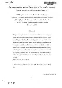
Methods involving continuous system simulation and feedback principles In contrast to the methods which are based on discrete models, the most widely used approach to inverse simulation involving continuous system simulation principles avoids iterative methods of solution and involves the use of a feedback approach. This can be linked to methods used in the past for divider units and inverse function generators in electronic analogue computers. Some early applications involving the feedback approach to inverse simulation can be found in work carried out at the DLR aerospace research institute in Germany.6,7. A similar approach, termed ‘inverse dynamics compensation via simulation of feedback control systems’ (IDCS) was developed by Tagawa and Fukui8,9 and further developments and applications involving feedback-based methods have been reported more recently 10 – 13. The feedback approach to inverse simulation may be explained most easily using linear models and analysis based on the use of Laplace transforms. The block diagram shown in Figure 1 involves a single-input single-output linear model G(s) and a feedback loop with a cascaded transfer function block K(s). The transfer function relating the variable W(s) in this block diagram to a reference input V(s) is given by: ( ) ( )
= ( )
( )
(1)
If 1/K(s) is small compared with the magnitude of G(s) the transfer function may be approximated by: ( ) ( )
≈
(2)
( )
Thus, if K(s) simply involves a gain factor, the transfer function W(s)/V(s) can be made to approximate very closely the inverse model, provided the chosen gain factor is sufficiently large. It should be noted, however, that although simple high-gain feedback is often found to provide accurate inverse solutions, the approach is not limited to this form of proportional control and more complex forms of K(s) may sometimes be useful.
3
w(t) – the output variable from the inverse simulation
v(t) – the variable representing the desired output from the inverse simulation
K
G
+
-
Figure 1. Block diagram illustrating the principle of inverse simulation based on the use of feedback (with variables shown as functions of t rather than the Laplace variable s). The given linear or nonlinear model is represented by the block G. For large values of the gain factor K, the variable w(t) closely approximates the input to the model G required to produce an output from that model that matches the reference input time history v(t). The form of this block diagram conforms to standard conventions used in control systems engineering. It is important to note that the feedback approach does not provide a unique inverse simulation. The high-gain cascaded block K(s) that is introduced within the feedback loop can have many different forms and has a structure and parameter values that must be chosen by the user. However, provided the feedback gain factor values are large over the complete frequency range of importance, the overall properties of the inverse simulation model are insensitive to the precise parameter values used and the feedback structure provides a close approximation to the true inverse model. It is also important to note that, although the feedback approach has been justified here using linear systems analysis methods for a singleinput single-output system model, extensive experience with problems involving a range of different aircraft, ship and process systems has demonstrated that it can also be used successfully with more complex nonlinear and multi-input multi-output descriptions.
4
The need to design a feedback system in creating the inverse simulation might be considered as a disadvantage compared with iterative methods based on discrete models. However, the feedback design issue need not form a barrier since it is, in general, significantly easier to obtain the feedback structure for an inverse simulation than to design a conventional feedback control system of similar complexity. This is because the development of an inverse simulation model for a given forward model involves the application of feedback to a system with precisely known dynamics. In addition, the inverse simulation involves no external disturbances and no measurement noise, unlike most practical situations where feedback system design methods are used for control system design. Therefore, for the purposes of inverse simulation, some very simple methods of feedback system design based on high gain solutions can be applied without difficulty, although techniques of this kind would be considered unsuitable for most practical control system design problems. The application of inverse simulation to train performance analysis. The train performance model The mathematical basis for train perfomance system modelling is well established and is based largely on the work of Davis14. A report by Lukaszewicz15 includes a useful and comprehensive review of more recent theoretical and experimental work relating to train performance models which, conventionally, are based on a one-dimensional model in the form of a set of ordinary differential equations and algebraic equations representing the characteristics of the traction system, vehicles and route. Since the model is generally nonlinear in form, analytical methods of solution are inappropriate except in some special cases. Numerical methods of solution are therefore necessary and there are many published accounts of investigations involving computer-based modelling of train performance. Studies have also been published involving comparisons of simulation model results with measured data from train performance tests for equivalent conditions and have demonstrated the validity of the computer-based modelling approach (see e.g. [15]). For development work, continuous system simulation tools can have significant benefits in terms of robustness and transparency compared with approaches involving general-purpose programming languages. Examples of such tools include the commercially-supported MATLAB® software16 and its associated Simulink® graphical environment16, or the broadly-similar open-source Scilab17 software. One significant advantage of software development tools of this kind is that they allow use of well-proven numerical routines for the solution of ordinary
5
differential equations and related tasks associated with simulation development. They also provide a well-documented development environment, both for the simulation aspects of the work and for the associated tasks involving data manipulation 16-18. In lumped-parameter mathematical models conventionally used for train-performance investigations, the distance travelled as a function of time, x(t), is normally considered as one of the output quantities, along with the velocity 𝑥̇ (𝑡) and the acceleration 𝑥̈ (𝑡). For simplicity the vehicles forming the train may be regarded as a single mass which is acted upon by a number of distinct forces. These include the tractive force, braking force, a gravitational force associated with gradients and forces representing other components of the resistance to motion. The resulting one-dimensional equation of motion has the general form: 𝑀(1 + 𝜙)𝑥̈ (𝑡) = 𝐹 (𝑡) − 𝐹 (𝑡) − 𝑅(𝑥̇ (𝑡)) ± 𝑀𝑔 sin 𝛼(𝑥(𝑡))
(3)
where 𝐹 (𝑡) and FB(t) are the tractive force and braking force. The variable 𝑅(𝑡) is the velocity-dependent resistance to motion, M is the mass of the train, 𝑔 is the acceleration due to gravity, 𝜙 is a rotational mass factor introduced to allow for the effects of rotational inertia and 𝛼 is the track gradient angle which, of course, is dependent on the train position x(t). The complete term 𝑀 (1 + 𝜙) is conventionally referred to as the ‘dynamic mass’. The resistance 𝑅(𝑥̇ ) in (3) involves three constants, 𝐴 , 𝐵′ and C which have to be estimated empirically for the specific vehicles being considered, giving an overall expression of the form: 𝑅 = 𝐴 + 𝐵′𝑥̇ + 𝐶𝑥̇
(4)
where 𝐴 and 𝐵 depend on the mass M and the coefficient C depends on aerodynamic factors. It should be noted that although curvature effects are not incorporated in this model they could be included without difficulty and would introduce an additional resistance term dependent on train position for the chosen route. It should also be noted in (3) that, in practice, the terms FT and FB are such that when the tractive force term FT has a non-zero value the braking force FB is zero and, correspondingly, when the braking force FB has a non-zero value the tractive force FT is zero. The power P is given by the equation
6
(5)
𝑃 = 𝑇𝑥̇
where T is the instantaneous tractive force. This equation shows that for a constant level of power the available tractive force falls as the speed increases. In addition, it is assumed that at low speed, until the train speed reaches a specific value Vch, the available tractive force may be limited to a value T0 to ensure that adhesion between the driven wheels and the rails is maintained, even under adverse environmental conditions. The corresponding energy consumption E over the period from the start t= 0 to time t= τ is given by: 𝐸 = ∫ 𝑃𝑑𝑡 (6) Braking action is included in the simulation model using a very simple type of representation. The braking thrust is assumed to be frictional and is taken to be numerically equal, but opposite in sign, to the tractive force applied at low speeds, T0. This negative thrust value is applied continuously from initiation of the braking phase until the train speed reaches zero. At that time instant the thrust, resistance and gradient terms in the basic equation of motion are all switched to zero to ensure that no further movement can occur in the simulated system. Regenerative braking action could be included in the simulation model without difficulty and is of particular interest in terms of the possible application of inverse simulation to questions of energy usage. Since the simulation model must accommodate speed restrictions, a feature has been included which allows for a transition to a speed-limited condition as the train accelerates. This may be regarded as a simplified representation of driver action. Speed at each instant of time is compared with the defined limiting value for the point on the route at which the train is operating and a time-varying factor Cds(t) is introduced. If the speed is above the limit this factor is set to zero, while if the speed is below the limit by a value vd (or more), the factor Cds(t) is given a value of unity. Between these critical speed values Cds(t) varies with train speed between 0 and 1 in a linear fashion, as shown in Figure 2. The the tractive force value at each time step in the simulation is multiplied by the factor Cds(t) to represent driver control actions in approaching and adhering to the speed limit. The tractive force is thus taken from the steady value used just before the speed limit, through a steadily falling range of values as the limit is approached, to a value of zero when the speed
7
becomes equal to or greater than the limiting value. Other methods for including driver control action could be considered, but this was thought to be an appropriate, simple and easily-implemented approach. Situations involving other forms of speed restriction can be handled in a similar way within the simulation model. Braking action could also be introduced during the approach to a speed restriction by using a method similar to that outlined above for implementation of the braking phase.
Factor Cds
vd
1.0
0.0 Speed limit
Train speed
Figure 2. Diagram illustrating the method used in the train simulation model to take account of speed limits. Verification of the inverse simulation approach In order to illustrate the use of these concepts for the train application it is useful to consider a simple example in which output variables from a conventional forward simulation model are applied as input variables to a corresponding inverse simulation model. If the inverse simulation model is correct this should, of course, generate the time history of inputs applied to the original forward simulation. As well as providing verification of the inverse simulation concept, this process can also provide useful insight about implementation of the inverse simulation method.
8
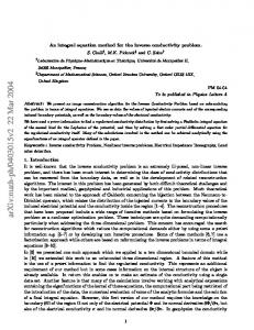
Figure 3 is a block diagram which illustrates the basis of the verification process. The inverse simulation model is represented in the lower part of the diagram and shows the feedback loop. This negative feedback path can, in principle, involve either position or velocity feedback as the primary feedback variable since the inverse model can be driven either from a time history of required distance values or a corrresponding time history of required velocity values. In the case shown in Figure 3, the input to the inverse simulation model is the required distance time history and this is generated using the forward simulation model. In normal applications of the inverse approach the time history used as input to the inverse simulation would be generated in some other way, but the use of this cascade arrangement of forward and inverse simulation models allows us to establish the validity, or otherwise, of the method. If the approach is valid the power or thrust time history found at the output of the inverse simulation model should be very close to the time history of the power or thrust input originally applied to the forward simulation model. Forward simulation model Time history of Power/thrust input
Train simulation model (including limits)
Predicted velocity Predicted distance
Inverse simulation model
+ -
Gain Factor K(s)
Predicted power/ thrust
Train simulation model (without limits)
9
Velocity Distance
Figure 3. Block diagram of the cascade arrangement of forward and inverse simulation models used for testing the inverse simulation approach. In this case the primary feedback variable is the distance travelled but it should be noted that, in practice, there may be a subsidiary velocity feedback path involving feedback of the speed. This use of velocity feedback allows damping of transients that would otherwise be present in the main feedback loop. In general, the gain factor K(s) may therefore be throught of as involving more than one feedback pathway. It should be noted, also, that the model used for the inverse simulation does not involve limits (such as the tractive force limit T0 ). The specific case considered is representative of practice in the United Kingdom and involves a model of a Class 390 9-car Virgin West Coast Pendolino set. The data used for the model (Table 1) were obtained from annexes to a UK Rail Safety and Standards Board Report19. The tractive force limiting incorporated at low speeds involves a maximum tractive force of T0 when the train speed is below a specified value Vch . Route information has been created for this example and the chosen gradient profile involves level track for an initial distance xG and then a constant rising gradient of 1 in Y for the remainder of the route. The route has no significant curves so that curvature resistance can be neglected. There is an overall speed restriction in terms of a line-speed limit of Vmax.. The length of the route has been chosen to be relatively short, but includes four distinct phases of operation to be observed in the simulation – a) the initial acceleration to the maximum allowed speed, b) a steady-state phase involving a spell of continuous operation at that linespeed limit, but with a change of gradient, c) a coasting phase and d) a final braking phase to bring the train to rest. In the example being considered the coasting phase begins at a distance xC from the start and the braking phase at a distance xB. The value of the parameter vd, (which defines the speed difference at which driver action is initiated when approaching a speed limit location) was chosen to be 1 ms-1 (3.6 km/hour) for this example as the only limit involved is the overall line speed limit. Other numerical values for vd might be more appropriate for other forms of speed restriction.
10
Table 1. Parameter values used in simulation model for Class 390 9-car set and chosen route characteristics Quantity
Symbol
Maximum power
P
5070 kW (nominal maximum)
Train mass
M
530300 kg
Rotational mass factor
ϕ
0.08
Tractive force at zero speed
T0
200000 N
Upper limit of speed for tractive force limiting
Vch
25 ms-1
First resistance term
A’
5311 N
Second resistance term
B’
78.1056 Nm-1s
Third resistance term
C
11.7897 Nm-2s2
Line speed limit
Vmax
11
Numerical value with units
55.56 ms-1 (125 mph)
Gradient factor
Y
50
Distance at which gradient starts
xG
20,000 m
Distance at which coasting phase starts
xC
25,000 m
Distance at which braking phase starts
xB
28,000 m
Acceleration due to gravity
g
9.81ms-2
Figure 4 shows the characteristic curves for tractive force at the rail, T (kN), and resistive force at the rail R (kN) as a function of velocity 𝑥̇ (ms-1). The limiting value of tractive force of 200 kN at low speeds is clearly seen from these plots, together with the balancing speed (slightly greater than 70 ms-1) at which the tractive force is equal to the resistive force.
12
Figure 4. Characteristic curves for Pendolino 9-car set for parameter values of Table 1 in terms of the (continuous line) tractive force T (kN) and (dashed line) resistive force (kN) plotted against train speed (ms-1).
The forward and inverse simulation programs were written in MATLAB® code using standard MATLAB® ‘ode’ routines for solution of the ordinary differential equations16,18. Several different ode routines are available within MATLAB® and all the results presented here involved use of the low-order ode23 routine which is based on a Runge-Kutta type of
13
algorithm. Compared with some other available MATLAB® routines, this has relatively low accuracy but has advantages in terms of speed of solution. The form of feedback required in the inverse simulation model depends on the type of reference input being applied and this can be either a desired distance or desired velocity time history. Typical output variables obtained from the inverse simulation are the thrust or power time histories to provide the given desired distance or velocity time history used as input. Selection of the form and numerical values of parameters in block K(s) in the feedback pathways is a relatively straightforward process and, for many inverse simulation applications, may be approached using a trial and error procedure. Cases involving feedback from more than one output variable can be better handled using simple analysis and design tools from feedback control theory, such as root locus design methods or eigenstructure assignment. For this particular application the numerical value of the gain factors within K(s) depends on the form of input being applied to the inverse simulation model and whether the input to the train simulation block within the feedback loop is tractive force or power. The most obvious case of practical importance involves appplication of a distance versus time curve as input to the inverse simulation model. However, simple analysis for this situation suggested that use of a single gain factor in a distance feedback loop could result in high frequency oscillatory transients. In situations of this kind, involving oscillatory or even unstable responses in feedback systems, the use of a subsidiary rate-feedback pathway is a wellestablished control system design approach. However, in this application involving the train model, simple linear analysis shows very clearly that instability due to feedback is not an issue of practical importance, although damped oscillatory transient responses may be present for the variables within the inverse simulation. For this inverse simulation application a suitable feedback equation involves the introduction of a subsidiary feedback pathway based on the velocity variable from the inverse simulation model, 𝑥̇ , in addition to the primary feedback loop involving the difference between the required distance, 𝑥 , and the corresponding distance, 𝑥 , from the inverse model. For the case of the thrust variable, the feedback equation has the form: 𝑇
= 10 𝑥
−𝑥
− 10 𝑥̇
14
(7)
where the gain factors of 10 in the main feedback loop and 10 in the subsidiary rate feedback pathway are chosen by the user and 𝑇 is the tractive force predicted by the inverse simulation model. A subsidiary feedback pathway involving the acceleration variable was also investigated as an alternative to the feedback equation shown in (7). This was found to give similar results but involved increased computational overheads and therefore was not adopted. As outlined above, a conventional forward simulation was first used to generate distance versus time curves for the given train set operating over the given route. The resulting data were used to form inputs for testing of the inverse simulation model, as shown in the block diagram of Figure 3. Figure 5 shows a plot of tractive force versus time for the forward simulation run. The initial phase shows the tractive force at the adhesion limit of 200 kN. When the speed reaches an appropriate value the tractive force starts to fall, following the characteristic hyperbolic curve for constant power conditions, as defined by (5), until the line-speed limit of 200km/hr is reached at about t = 240 s from the start. The tractive force is then reduced to a value of about 45 kN in order to observe the speed limit and this condition continues until the rising gradient is encountered at about t = 450 s (20 km from the start). The tractive force required to try to maintain the given line speed of 200 km/hr is then seen to increase in a stepwise fashion and continues to increase more or less linearly with time until the 25 km point is reached (about 550 s from the start) when coasting begins and the applied tractive force drops to zero. At 28km the braking phase starts, with a constant thrust of -200 kN applied. The train comes to a halt 680 s from the start, at a distance of about 29 km.
15
Figure 5. Plot of tractive force (N) applied as input for the forward simulation run versus time (s). Figure 6 is the corresponding curve for train speed versus time. It is interesting to note the reduction in speed which occurs at the start of the 1 in 50 gradient, which is encountered at 20 km (at about 450 s). It should be noted that the negative acceleration during the coasting and braking phases is affected by the rising gradient during those phases of operation. The braking phase involves a constant acceleration of -0.55ms-2 (approximately 5 % g) and this represents a relatively modest brake application.
16
Figure 6. Plot of speed (ms-1) versus time (s) for the forward simulation run.
Figure 7 shows a plot of distance travelled versus time and this is entirely consistent with the results in Figure 6. Figure 8 shows the power usage during the first three phases of the simulation, together with braking power appled in the final phase.
17
Figure 7. Plot of distance travelled (m) versus time (s) for the forward simulation run.
18
Figure 8. Plot of power (MW) versus time (s) corresponding to the tractive force and speed curves of Figure 5 and 6. Note the negative values of power in the final braking phase. Results for the tractive force obtained by inverse simulation involving application of the distance versus time record of Figure 7 as input are almost identical to the original tractive force input values applied to the forward simulation (Figure 5). The numerical differences between the forward and inverse tractive force time histories involve steady-state values very close to zero, together with short transients whenever large changes of tractive force occur, as shown in Figure 9. The precise form of these transient errors are dependent on the gain factors used within the feedback loop for the inverse simulation but the errors are small in
19
relation to the dynamic range of the variables involved. The detail of these transients may be seen in Figure 10 which shows the form of the transient occurrring at the transition from constant speed running to coasting for the specific gain factors of (7). It may be seen that this oscillatory transient is of short duration, has peak values approximately one tenth of the maximum tractive force applied and has a mean value which is approximately zero. It can be shown that if the tractive force time history obtained using the inverse simulation is then applied as input to the forward simulation, the tractive force transient errors have negligible effect on the values of speed and distance travelled.
Figure 9. Time history plot showing difference between the tractive force (N) applied as input for the forward simulation (as shown in Figure 5) and the corresponding tractive force (N) found by inverse simulation using the distance/time data of Figure 7 as input.
20
Figure 10. Detail of a typical transient within the plot of Figure 9 showing the difference between tractive force values used in the forward simulation and corresponding values found from the inverse simulation.
21
Results from inverse simulation applications The results presented above provide verification of the feedback approach for generation of an inverse simulation model for the case considered. Very similar results have been obtained with other feedback structures and gain factor values and for different train and route configurations. Although results presented above are important in terms of the development of the inverse simulation methodology, it is also necessary to consider how results of practical interest might be obtained from an inverse model of this type. One obvious use of the inverse simulation would be to investigate how tractive force or power requirements would change when the time required for the journey is changed. This could provide useful and very direct insight about the achievability, or otherwise, of proposed schedule changes, together with information about driving strategies and possible energy savings. For example, one simple investigation could involve using the distance-time data shown in the plot of Figure 7 and increasing or decreasing the journey time values by a specific amount without altering the corresponding distance values.
22
Figure 11. Plot of tractive force (N) versus time (s) found from inverse simulation with distance/time record of Figure 7 applied as input but with all time values increased by 5 %. Figure 11 shows results in terms of the tractive force for a case where the journey time was increased by 5% overall, with a corresponding increase in time values over all stages of the record. This shows clearly that, compared with the previous case, the tractive force and braking force time histories have changed significantly. For example, the initial tractive force has fallen from 200×105 N to a value of about 180×105 N and the tractive force values used in some other sections have also been reduced. One section of the route for which the tractive force has increased slightly is in the coasting section where, due to the rising
23
gradient, some thrust is required to maintain the given schedule over this section of the route for the initial conditions that apply at the start of that section. Figure 12 shows results from the inverse simulation involving a distance/time schedule where times have been reduced by 5% compared with the profile shown in Figure 7. Here, as would be expected, the tractive force and braking force values found from the inverse simulation have been increased to satisfy the new timing requirement and some values, such as the initial value of tractive force, clearly exceed the specified maxima. In addition, the “coasting” phase in this case involves a small negative tractive force to ensure that the schedule is matched, equivalent to a very mild brake application. It may also be seen that the final braking force has been increased to ensure that train comes to a halt at the required point. The speed/time profile shown in Figure 13 indicates that the reduced time schedule leads to a cruise speed which slightly exceeds the 200 km/hr (55.56 m/s) line limit.
24
Figure 12. Plot of tractive force (N) versus time (s) found from inverse simulation with distance/time record of Figure 7 applied as input but with all time values reduced by 5%.
Figure 13. Plot of speed (ms-1) versus time (s) obtained from the inverse simulation model for the case corresponding to the results of Figure 12. It is of interest also to compare energy usage figures for the three schedules considered. Using the simulation records involving the section from the start until the point at which coasting began, the first case gave a value of 2.16 × 10⁹ Ws (0.60 MWhour) and this was found to fall to a value of 2.03× 10⁹ Ws (0.56 MWhour) when the slowest schedule was considered, involving a 5% increase in the scheduled time compared with the first case.
25
Similarly, the energy usage for the third case, involving a scheduled time that was 5% shorter than the schedule for the first case, was 2.32 × 10⁹ Ws (0.64 MWhour). Thus it can be seen that a 5% reduction in journey time for this specific section of the route led to an increase in energy usage of 7.2%. The slowest schedule was found to require 12.3% less energy than the fastest. Discussion It is clear from the results above that the feedback method of inverse simulation, in which we start from a record of the required distance versus time and obtain the necessary tractive force or power to satisfy that performance requirement, is a valid approach. It provides an alternative to conventional forward simulation methods where the starting point is the applied tractive force or power and the simulation is used to find the corresponding values of speed and distance travelled at each time point. As shown in Figures 10 and 11, one way in which this inverse formulation could be applied is in determining how performance is limited by the available tractive force or power. Since energy usage may be found from the integral of power with respect to time, this approach also allows investigation of the costs and benefits of using different schedules and the effects of coasting in terms of energy savings. Although a simplified form of train model has been used here to illustrate this inverse simulation approach, any other train performance model could be used in the same way. Sensitivity analysis in terms of the effect of changes in train parameters (such as mass, resistance or braking characteristics) on tractive force, power or energy usage, is another obvious application. Investigation of the potential benefits and possible costs of introducing regenerative braking provides a further possible application area, using an appropriately modified train model. Similarly, for the design of new metro type routes involving frequent stops in a relatively short distance, inverse simulation could be a useful tool for investigating possible energy savings through the introduction of gradients before and after intermediate stations to provide a natural resistive force as the station is approached and a natural accelerating force when the train starts again. Conventional forward simulation methods have, of course, been used for this type of applications in the past but the inverse approach should allow more direct analysis and, perhaps, new insight in investigating such issues.
26
It should be noted that it is possible to introduce constraints into the inverse simulation program so that use of tractive force or power values outside an allowed range is prevented. This could, for example, be used to eliminate the possible use of tractive force values at low speeds that exceed the maximum for maintaining adhesion or to introduce an upper limit on the braking force applied. However, the use of hard constraints of this kind can introduce numerical problems in terms of the accurate detection of the time at which a limit occurs and might require the use of more specialised numerical techniques within the simulation, possibly at some cost in terms of computational efficiency and thus speed of solution20. In addition, it should be noted that the use of very large values of gain within the feedback loops for the inverse simulation may, in some situations, lead to issues of excessive “stiffness” in the equations defining the inverse model 18, 20. Specialised integration algorithms may then be needed which are suitable for sets of stiff ordinary differential equations. However, a combination of a stiff model and hard nonlinearities can be difficult to deal with efficiently. Information available from other inverse simulation applications may point to methods for handling such situations if they arise 10-13. The choice of input for an inverse model is an issue of considerable importance. The example considered above involved application of a distance versus time curve as input to the inverse simulation model. An alternative would be a speed versus time curve. Although use of that latter form of input was found to provide inverse simulation results that were virtually identical to those obtained using the distance versus time input for the high gain values being used in the feedback loops, it was considered that the use of the speed input is less realistic in practical terms since train schedules are normally defined in terms of distance travelled versus time. A further advantage of using the distance input can be deduced from feedback systems theory, since it can be shown (using linear systems analysis methods) that a primary feedback loop involving the distance variable rather than the speed variable gives, theoretically, zero steady state distance error in the inverse simulation. On the other hand, the use of the speed variable in the primary feedback loop would give rise to a steady state speed errors in the inverse simulation, although this could be made negligibly small through use of a large gain factor in the primary feedback loop. Another possible approach would involve defining the schedule in terms of speed versus distance travelled but this introduces additional complications because the basic train model involves a set of ordinary differential equations involving time as the independent variable. In this context, it is interesting to consider the approach to the choice of inputs for inverse simulation which has been adopted in the helicopter flight simulation field where standard
27
forms of input have been developed based on polynomials which represent potentially achievable manoeuvres3. In a similar way, separate polynomial-based input time histories could be developed to describe desirable curves for different phases of a typical train performance record. In the context of the simple example considered in this paper there could be separate polynomial descriptions for the initial acceleration phase, the transition to a constant speed condition, coasting and braking. These could then be combined to define a complete distance versus time curve which could provide the input to determine the corresponding tractive force time history. A related topic, which should also be considered for further investigation, concerns the fact that an envelope of possible performance curves may be needed, rather than a single curve specifying a single required time history. Although it has been emphasised that the design of feedback systems for implementation of the inverse simulation method presented here is simpler than the design of equivalent feedback control systems, since there are no uncertainties or unmeasured disturbances in the system around which feedback is applied, this should not be taken as implying that the forward model and the inverse model do not themselves involve uncertainties and imperfections. Model uncertainties and inherent simplifications mean that model validation issues remain important in inverse simulation, just as they are in conventional forward simulation. Hence, in any application of inverse simulation methods, it is always necessary to consider the sensitivity of inverse simulation results to assumptions, simplifications, uncertainties and possible errors in the representation of the train and the route. Although the application of inverse simulation to train performance investigation is clearly at an early stage, the feedback approach to inverse simulation has already been considered in at least one other railway-related application. That involves monitoring of track irregularities using a dynamic vehicle suspension model in a development which is intended allow rail surface irregularities to be found from measured vehicle responses21. Conclusions As stated in the introductory section, the main objective of this paper is to introduce inverse simulation methods in the context of train performance simulation problems and to demonstrate the validity of the approach through an illustrative example. In that example one specific method of inverse simulation has been applied and has been shown, by means of a verification process involving use of the corresponding traditional forward simulation in cascade with the inverse simulation, to provide a correct and useful inverse model.
28
Conventional forward simulation models have been extensively validated in the past through comparisons with data recorded during train performance testing programmes. This study has therefore focussed on the generation of an inverse simulation model equivalent to these accepted forms of forward simulation model and on verification of the inverse simulation methodology. The evidence presented in earlier sections of the paper shows clearly that inverse simulation methods are potentially useful for the investigation of train performance and that the example demonstrates both the correctness of the inverse simulation method being considered and some possible applications. The inverse simulation approach does not replace conventional simulation methods but provides insight that is distinctly different and forms an alternative to the more standard simulation approaches currently in use. The method of inverse simulation based on the properties of feedback systems presented in this paper is simple to apply. Although inverse models obtained in this way are not unique and results obtained depend on the form of feedback structure and gain factors applied, the method has been shown to provide a valid approach to inverse simulation for train performance analysis applications. Comparisons of results presented here with results obtained using other methods of inverse simulation would be useful and could be an interesting area for future research. Further work is also necessary to develop the approach into one that can be used in a routine way for practical train performance applications using more accurate train models and information for specific routes. Declaration of conflicting interests The author declares that there is no conflict of interest in terms of the work carried out in preparing this paper or in terms of the information presented. References 1. Hess RA, Gao C and Wang SH. A generalized technique for inverse simulation applied to aircraft maneuvers. AIAA J. Guidance Control and Dynamics. 1991; 14 (5): 920-926. 2. Thomson DG and Bradley R. The principles and practical application of helicopter inverse simulation. Simulation Practice and Theory. 1998; 6 (1): 47-70.
29
3. Thomson D and Bradley R. Inverse simulation as a tool for flight dynamics researchPrinciples and applications. Prog. in Aerospace Sciences. 2006; 42: 174-210. 4. Lu L, Murray-Smith DJ and Thomson DG. Issues of numerical accuracy and stability in inverse simulation, Simulation Modelling Practice and Theory. 2008; 16: 1350-1364. 5. Thomson DG and Bradley R. Development and verification of an algorithm for helicopter inverse simulation. Vertica. 1990; 14(20): 185-200. 6. Hamel PG. Aerospace vehicle modelling requirements for high bandwidth flight control. In, Cook MV and Rycroft MJ (eds.), Aerospace Vehicle Dynamics and Control, Oxford, UK; Clarendon Press: 1994, pp. 1-31 7. Buchholz JJ and von Grünhagen W. Inversion Impossible?. Bremen, Germany: University of Applied Sciences, Technical Report, 2004. 8. Tagawa Y and Fukui K. Inverse dynamics calculation of nonlinear model using low sensitivity compensator. In: Proc. of Dynamics and Design Conf. 1994, pp. 185-188. 9. Tagawa Y, Tu JY and Stoten DP. Inverse dynamics compensation via ‘simulation of feedback control systems’. Proc. Institution of Mechanical Engineers, Part I: J. Systems and Control Eng.. 2012; 225: 137-153. 10. Murray-Smith DJ. Feedback methods for inverse simulation of dynamic models for engineering system applications, Mathematical and Computer Modelling of Dynamical Systems. 2011; 17 (5): 515-541. 11. Murray-Smith DJ. Inverse simulation and analysis of underwater vehicle dynamics using feedback principle, Mathematical and Computer Modelling of Dynamical Systems. 2014; 20 (1): 45-65. 12. Murray-Smith DJ and McGookin EW. A case study involving continuous system methods of inverse simulation for an unmanned aerial vehicle application, Proceedings Institution of Mechanical Engineers, Part G: J. Aerospace Eng. 2015; 229(14): 27002717. 13. Murray-Smith DJ. Modelling and Simulation of Integrated Systems in Engineering. Cambridge, UK; Woodhead: 2012, Chapter 4 14. Davis WJ Jr. The tractive resistance of electric locomotives and cars. General Electric Review, 1926; 29 (10): 685-707. 15. Lukaszewicz P. Energy Consumption and Running Time for Trains, Doctoral thesis, Royal Institute of Technology, Stockholm, Sweden, 2001. https://pdfs.semanticscholar.org/b2a1/478bb878493fb4eee06e89f847d80e649309.pdf (accessed 22 December 2016). 16. Mathworks Inc. MATLAB®/Simulink® modelling and simulation software. http://www.mathworks.com/products/. (accessed 22 December 2016).
30
17. Campbell SL, Chancelier J-P, Nikoukhah, R. Modeling and Simulation in Scilab/Scicos, New York, NY, USA; Springer: 2000. 18. Lindfield G and Penny J. Numerical Methods Using MATLAB, Hemel Hempstead, UK; Ellis Horwood: 1995 19. Anon. T712 Report. Research into Trains with Lower Mass in Britain: Quantification of the Benefits of Train Mass Reduction. Annex E1. London, UK, Rail Safety and Standards Board Ltd., August 2010. 20. Murray-Smith DJ. Continuous System Simulation, London, Chapman and Hall, 1995, Section 4.7. 21. Schenkendorf R and Groos J. Global sensitivity analysis applied to model inversion problems: a contribution to rail condition monitoring. International Journal of Prognostics and Health Management. 2015; 6: 14 pp. https://www.phmsociety.org/sites/phmsociety.org/files/phm_submission/2015/ijphm_15_0 19.pdf (accessed 22 December 2016).
31