Jul 7, 2015 - Y -box), an operator for synchronization (the sync node), and a primitive ...... represented with a Y-combinator: while this is fine in call- by-name ...
Parallelism and Synchronization in an Infinitary Context Ugo Dal Lago
Claudia Faggian
Benoˆıt Valiron
arXiv:1505.03635v2 [cs.LO] 7 Jul 2015
Univ. di Bologna & INRIA CNRS & Univ. Paris Diderot CentraleSup´elec & LRI, Univ. Paris Sud
Abstract—We study multitoken interaction machines in the context of a very expressive linear logical system with exponentials, fixpoints and synchronization. The advantage of such machines is to provide models in the style of the Geometry of Interaction, i.e., an interactive semantics which is close to lowlevel implementation. On the one hand, we prove that despite the inherent complexity of the framework, interaction is guaranteed to be deadlock-free. On the other hand, the resulting logical system is powerful enough to embed PCF and to adequately model its behaviour, both when call-by-name and when call-byvalue evaluation are considered. This is not the case for singletoken stateless interactive machines.
I. I NTRODUCTION What is the inherent parallelism of higher-order functional programs? Is it possible to turn λ-terms into low-level programs, at the same time exploiting this parallelism? Despite great advances in very close domains, these questions have not received a definite answer, yet. The main difficulties one faces when dealing with parallelism and functional programs are due to the higher-order nature of those programs, which turns them into objects having a non-trivial interactive behaviour. The most promising approaches to the problems above are based on Game Semantics [1], [14] and the Geometry of Interaction [12] (GoI), themselves tools which were introduced with purely semantic motivations, but which have later been shown to have links to low-level formalisms such as asynchronous circuits [10]. This is especially obvious when Geometry of Interaction is presented in its most operational form, namely as a token machine [7]. Most operational accounts on the Geometry of Interaction are in particle-style, i.e., a single token travels around the net; this is largely due to the fact that parallel computation without any form of synchronization nor any data sharing is not particularly useful, so having multiple tokens would not add anything to the system. While some form of synchronization was implicit in earlier presentations of GoI, the latter has been given a proper status only recently, with the introduction of SMLL [4], where multiple tokens circulate simultaneously, and also synchronize at a new kind of node, called a sync node. All this has been realized in a minimalistic logic, namely multiplicative linear logic, a logical system which lacks any copying (or erasing) capability and, thus, is not an adequate model of realistic programming languages (except purely linear ones, whose role is relevant in quantum computation [24]). Multitoken GoI machines are relatively straightforward to define in a linear setting: all potential sources of parallelism
Akira Yoshimizu Univ. of Tokyo
give rise to actual parallelism, since erasing and copying are simply forbidden. As a consequence, managing parallelism, and in particular the spawning of new tokens, is easy: the mere syntactical occurrence of a source of parallelism triggers the creation of a new token. Concretely, these sources of parallelism are unit nodes (when thought logically), or constants (when read through the lenses of functional programming). The reader will find an example in Section II, Fig. 1. But can all this scale to more expressive proof theories and programming formalisms? If programs or proofs are allowed to copy or erase portions of themselves, the correspondence between potential and actual parallelism vanishes: any occurrence of a unit node can possibly be erased, thus giving rise to no token, or copied, thus creating more than one token. The underlying interactive machinery, then, necessarily becomes more complex. But how? The solution we propose here relies on linear logic itself: it is the way copying and erasing are handled by the exponential connectives of linear logic which gives us a way out. We find the resulting theory simple and elegant. In this paper we generalize the ideas behind SMLL in giving a proper status to synchronization and parallelism in GoI. We show that multiple tokens and synchronization can work well together in a very expressive logical system, namely multiplicative linear logic with exponentials, fixpoints, and units. The resulting system, called SMEYLL, is then general enough to simulate universal models of functional programming: we prove that PCF can be embedded into SMEYLL, both when call-by-name and call-by-value evaluation are considered. The latter is not the case for single-token machines, as we illustrate in Section II. This is a version extended with proofs and more details of an eponymous paper [5] which appeared in the proceedings of the Thirteenth Annual Symposium on Logic in Computer Science . Contributions This paper’s main contributions can be summarized as follows: • An Expressive Logical System. We introduce SMEYLL nets, whose expressiveness is increased over MELL nets by several constructs: we have fixpoints (captured by the Y -box), an operator for synchronization (the sync node), and a primitive conditional (captured by the ⊥-box). The presence of fixpoints forces us to consider a restricted
•
•
•
notion of reduction, namely closed surface reduction (i.e., reduction never takes place inside a box). Cuts can not be eliminated (in general) from SMEYLL proofs, as one expects in a system with fixpoints. Reduction, however, is proved to be deadlock-free, i.e., normal forms cannot contain surface cuts. A Multitoken Interactive Machine. SMEYLL nets are seen as interactive objects through their synchronous interactive abstract machine (SIAM in the following). Multiple tokens circulate around the net simultaneously, and synchronize at sync nodes. We prove that the SIAM is an adequate computational model, in the sense that it precisely reflects normalization through machine execution. The other central result about the SIAM is deadlock-freeness, i.e., if the machine terminates it does so in a final state. In other words, the execution does not get stuck, which in principle could happen as we have several tokens running in parallel and to which we apply guarded operators (e.g., synchronization). Our proof comes from the interplay of nets and machines: we transfer termination from machines to nets, and then transfer back deadlock-freeness from nets to machines. A Fresh Look at CBV and CBN. A slight variation on SMEYLL nets, and the corresponding notion of interactive machine, is shown to be an adequate model of reduction for Plotkin’s PCF [22]. This works both for call-byname and call-by-value evaluation and, noticeably, the same interactive machine is shown to work in both cases: what drives the adoption of each of the two mechanisms is, simply, the translation of terms into proofs. What is surprising here is that CBV can be handled by a stateless interactive machine, even without the need to go through a CPS translation. This is essentially due to the presence of multiple tokens. New Proof Techniques. Deadlock-freeness is a key issue when working with multitoken machines. A direct scheme to prove it (the one used in [4]) would be: (i) prove cut elimination for the nets, (ii) prove soundness for the machine, and (iii) deduce deadlock-freeness from (i) and (ii). However, in a setting with fixpoints, cut elimination is not available because termination simply does not hold1 . Instead, we develop a new technique, which heavily exploit the interplay between net rewriting and the multitoken machine. Namely, we transfer termination of the machine (including termination as a deadlock) into termination of the nets. This combinatorial technique is novel and uses multiple tokens in an essential way. It appears to be of technical interest in its own.
Related Work Almost thirty years after its introduction, the literature on GoI is vast. Without any aim of being exhaustive, we only mention the works which are closest in spirit to what we are doing here. 1 Even without fixpoints, there is to the authors’ knowledge no direct combinatorial proof of termination for surface reduction.
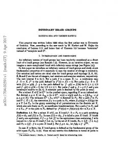
The fact that GoI can be turned into an implementation scheme for purely functional (but expressive) λ-calculi, has been observed since the beginning of the nineties [7], [17]. Among the different ways GoI can be formulated, both (directed) virtual reduction and bideterministic automata have been shown to be amenable to such a treatment. In the first case, parallel implementations [20], [21] have also been introduced. We claim that the kind of parallel execution we obtain in this work is different, being based on the underlying automaton and not on virtual reduction. The fact that GoI can simulate call-by-name evaluation is well-known, and indeed most of earlier results relied on this notion of reduction. As in games [2], call-by-value requires a more sophisticated machinery to be handled by GoI. This machinery, almost invariably, relies on effects [13], [23], even when the underlying language is purely functional. This paper suggests an alternative route, which consists in making the underlying machine parallel, nodes staying stateless. Another line of work is definitely worth mentioning here, namely Ghica and coauthors’ Geometry of Synthesis [8], [9], in which GoI suggests a way to compile programs into circuits. The obtained circuit, however, is bound to be sequential, since the interaction machinery on which everything is based is particle-style. On the side of nets, Y-boxes allow us to handle recursion. A similar box was originally introduced by Montelatici [19], even though in a polarized setting. Our Y-box differs from it both in the typing and in the dynamics; these differences are what make it possible to build a GoI model. II. O N M ULTIPLE T OKENS AND THE E XPONENTIALS In this section, we will explain through a series of examples how one can build a multitoken machine for a non-linear typed λ-calculus, and why this is not trivial. Let us first consider a term computing a simple arithmetical expression, namely M = (λx.λy.x + y)(4 − 2)(1 + 2). This term evaluates to 5 and is purely linear, i.e. the variables x and y appear exactly once in the body of the abstraction. How could one evaluate this term trying to exploit the inherent parallelism in it? Since we a priori know that the term is linear, we know that the subexpressions S = (4 − 2) and T = (1 + 2) are indeed needed to compute the result, and thus can be evaluated in parallel. The subexpression x+y could be treated itself this way, but its arguments are missing, and should be waited for. What we have just described is precisely the way the multitoken machine for SMLL works [4], as in Fig. 1 (left): each constant in the underlying proof gives rise to a separate token, which flows towards the result. Arithmetical operations act as synchronization points. Now, consider a slight variation on the term M above, namely N = (λx.λy.x+x)(4−2)(1+2). The term has a different normal form, namely 4, and is not linear, for two different reasons: on the one hand, the variable x is used twice, and on the other, the variable y is not used at all. How should one proceed, then, if one wants to evaluate the term in parallel? One possibility consists in evaluating subexpressions only if they are really needed. Since
M
add add 4 2 one one `
`
N in CBN
1 2 one one
ax ax
add cut
⊗
ax ax ?d ax
?d ?c
T
add S
?w
⊗ `
`
!
! cut
⊗
ax ⊗
Fig. 1. Actual vs. Potential Parallelism.
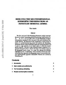
the subexpression x + x is of course needed (it is, after all, the result!), one can start evaluating it. The value of the variable x, as a consequence, is needed, and the subexpression it will be substituted for, namely 4 − 2, must itself be evaluated. On the other hand, 1 + 2 should not be evaluated, simply because its value does not contribute to the final result. This is precisely what call-by-name evaluation actually do. The interactive machine which we define in this paper captures this process. It has to be noticed, in particular, that discovering that one of the subexpressions is needed, while the other is not, requires some work. The way we handle all this is strongly related to the structure of the exponentials in linear logic. We give the CBN translation of N in Fig. 1 (right). The two rightmost subterms are translated into exponential boxes (where S is the net for 4 − 2 and T for 1 + 2), which serve as boundaries for parallelism: whatever potential parallelism a box includes, must be triggered before giving rise to an actual parallelism. Each of the occurrences of the variable x triggers a new kind of token, which starts from the dereliction nodes (?d) at the surface and whose purpose is precisely to look for the box the variable will be substituted for. We call these dereliction tokens. What happens if we rather want to be consistent with callby-value evaluation? In this case, both subterms (4 − 2) and (1 + 2) in the term N above should be evaluated. Let us however consider a more extreme example, in which call-by-name and call-by-value have different observable behaviors, for example the term L = (λx.1)Ω, where Ω = (λx.xx)(λx.xx). The call-by-value evaluation of L gives rise to divergence, while in call-by-name L evaluates to 1. Something extremely interesting happens here. We give the call-by-value translation of L in Fig. 2. First of all, we observe that a standard singleone 1
?w ?⊥
Ω
ax
ax
ax
?d
1
`
⊗
!
?d
Ω≡
Y ?d
cut
cut
Fig. 2. The CBV-translation of (λx.1)Ω.
token machine would start from the conclusion, find the node one, and exit again: such a machine would simply converge on the term L. When running on the term Ω alone, the machine would diverge, but as subterm of L, Ω is never reached, so
the machine’s behaviour on L is not the one which we would expect in call-by-value. Our multitoken machine, instead, simultaneously launches tokens from all dereliction nodes at surface: the dereliction token coming out of Ω (represented on the right in Fig. 2) reaches the Y-box, and makes the machine diverge. We end this section by stressing that the interactive machine we use is the same, and that this machine correctly models CBN and CBV, solely depending on the chosen translation of terms into nets. The call-by-name translation of L puts the subterm Ω in a box which is simply unreachable from the rest of the net (as in the case of T in Fig. 1), and our machine converges as expected. The call-by-value translation of L, on the other hand, does not put Ω inside a box. As a consequence, there is no barrier to the computation to which Ω gives rise— the same as if Ω would be alone—and our machine correctly diverges. This is the key difficulty in any interactive treatment of CBV, and we claim that the way we have solved it is novel. III. N ETS AND A M ULTITOKEN I NTERACTIVE M ACHINE We start with an overview of this section, which is divided into four parts. Nets and Their Dynamics: SMEYLL nets come with rewriting rules, which provide an operational semantics for them, and with a correctness criterion, which ultimately guarantees that nets rewriting is deadlock-free. Multitoken Machines: On any net we define a multitoken machine, called SIAM, which provides an effective computational model in the style of GoI. A fundamental property we need to check for the machine is deadlock-freeness, i.e., if the machine terminates it does so in a final state. From the beginnings of linear logic, the correctness criterion of nets has been interpreted as deadlock-freeness in distributed systems [3]; this is also the case for MELLS. Here, however, we work with surface reduction, and we have fixpoints. For these reasons, a rather refined approach is needed. The Interplay Between Nets and Machines: Nets rewriting and the SIAM are tightly related. We establish the following results. Let R denote a net, MR its machine, and the net rewriting relation. First of all, we know that (i) if R is cut-and-sync-free, the machine MR terminates in a final state. On the net hand, we establish that (ii) net rewriting is deadlock-free: if no reduction is possible from R, then R is cut-and-sync-free. On the machine side, we establish that (iii) if R S then MR converges/deadlocks iff the same holds for MS . We then use the multitoken paradigm to provide a decreasing parameter for net rewriting, and establish that (iv) if MR terminates, then R has no infinite sequence of reductions. Putting all this together, it follows that multitoken machines are deadlock-free. Computational Semantics: Finally, by using the machine representation, we associate a denotational semantics to nets, which we prove to be sound with respect to net reduction. A. Nets and Their Dynamics. In this section we introduce SMEYLL nets, which are a generalization of MELL proof nets. For a detailed account
on proof nets, we refer the reader to Laurent’s notes [15]: our approach to correctness, as well as the way to deal with weakening, is very close to the one described there. 1) Formulas: The language of SMEYLL formulas is identical to the one for MELL. The language of formulas is therefore: A ::= 1
|
⊥
|
X
|
X⊥
|
A⊗A
|
A`A
|
!A
|
is always finite. The sort of each node induces constraints on Multiplicatives A
A⊥ cut
B A B ⊗ ` A⊗B A`B Sync Units P1 . . . Pn one ⊥ 1 ⊥ ... P1 Pn Γ Exponentials and Fixpoints A ?A ?A Y ?c ?w ?d ! ?A ?A ?A !A ?A1 . . . ?An !A ?A1 . . . A⊥
?A,
where X ranges over a denumerable set of propositional variables. The constants 1, ⊥ are the units. Atomic formulas are those formulas which are either propositional variables or units. Linear negation (·)⊥ is extended into an involution on all formulas as usual: A⊥⊥ ≡ A, 1⊥ ≡ ⊥, (A⊗B)⊥ ≡ A⊥ `B ⊥ , (!A)⊥ ≡ ?A⊥ . Linear implication is a defined connective: A ( B ≡ A⊥ ` B. Atoms and connectives of linear logic are usually divided in two classes: positive and negative. Here however, we define positive (denoted by P ) and negative (denoted by N ) those formulas which are built from units in the following way: P ::= 1 | P ⊗ P , and N ::= ⊥ | N ` N . So in particular, there are formulas which are neither positive nor negative, e.g. ⊥ ` 1. 2) Structures: A SMEYLL structure is a finite labeled directed graph built over the alphabet of nodes which is represented in Fig. 3 (where the orientation is the top-bottom one). All edges have a source, but some edges may have no target; such dangling edges are called the conclusions of the structure. The edges are labeled with SMEYLL formulas; the label of an edge is called its type. We call those edges which are represented below (resp. above) a node conclusions (resp. premisses) of the node. We will often say that a node “has a conclusion (premiss) A” as shortcut for “has a conclusion (premiss) of type A”. When we need more precision, we distinguish between an edge and its type, and we use variables such as e, f for the edges. The nodes !, Y and ⊥ are called boxes. One among their conclusions (the leftmost ones in Fig. 3, which have type !A, !A and ⊥, respectively) is said to be principal, the other ones being auxiliary. !-boxes and Y-boxes are exponential. An exponential box is closed if it has no auxiliary conclusions. To each box is associated, in an inductive way, a structure which is called the content of the box. To the !-box we associate a structure with conclusions A, ?Γ. To the Y-box corresponds a structure of conclusions A, ?A⊥ , ?Γ. To the ⊥-box is associated a structure of non-empty conclusions Γ, together with a new node bot of conclusion ⊥. We represent a box b and its content S as in Fig. 4. With a slight abuse of terminology, the nodes and edges of S are said to be inside b. Similarly, a crossing of any box’s border is said to be a door, and we often speak of premiss and conclusion of a (principal or auxiliary) door. Note that the principal door of the Y-box (marked by Y) has premisses A, ?A⊥ and conclusion !A. A node occurs at depth 0 or at surface in the structure R if it is a node of R, while it occurs at depth n + 1 in R if it occurs at depth n in a structure associated to a box of R. Please observe that nets being defined inductively, the depth of nodes
ax A
A
?An
Fig. 3. SMEYLL Nodes.
!-box
Y-box
S A !A
!
... ? ... ? ?A1 ?An
S bot ... A ?A⊥ ⊥ Y ? ... ? ⊥ ⊥ !A ?A1 ⊥ ?An
⊥-box S ... Γ + ... + Γ
Fig. 4. SMEYLL Boxes.
the number and the labels of its premisses and conclusions, which are shown in Fig. 3. We observe that the ⊥-box is the same as in [11] and corresponds to the sequent calculus `Γ rule ` ⊥, Γ . All nodes are standard except sync nodes and Y-boxes, which need some further explanation: • Y-boxes model recursion (more on this when we introduce the reduction rules). Proof-theoretically, the Y-box corresponds to adding the following fix-point sequent calculus rule to MELL: ` A, ?A⊥ , ?Γ Y `!A, ?Γ •
Sync nodes model synchronization points. A sync node has n premisses and n conclusions; for each i (1 ≤ i ≤ n) the i-th premiss and the corresponding i-th conclusion are typed by the same formula, which needs to be positive.
Simple and positive structures. Two relevant classes of structures are simple and positive structures. A formula is simple it is is built out of {X, X ⊥ , 1, ⊗, `}. A structure R is simple (resp. positive) if all its conclusions are simple (resp. positive) formulas. This does not mean that all formulas occurring in R are simple (resp. positive). R can be very complex; the constraint only deals with R’s conclusions. 3) Correctness: A net is a structure which fulfills a correctness criterion defined by means of switching paths (see [15]). A switching path on the structure R is an undirected path2 such that (i) for each `-or-?c-node, the path uses at most one of the two premisses, and (ii) for each sync node, the path uses at most one of the conclusions. The former condition is standard, the latter condition rules out paths which bounce on sync nodes “from below”: a path crossing a sync node 2 By path, in this paper we always mean a simple path (no repetition of either nodes or edges).
may traverse one premiss and one conclusion, or traverse two distinct premisses. A structure is correct if: 1. none of its switching paths are cyclic, and 2. the content of each of its boxes is itself correct. The reader familiar with linear logic correctness criteria did probably notice that the only condition we require is acyclicity, and that connectedness is simply not enforced (as, e.g., in Danos and Regnier’s criterion [6]). Actually, the only role of connectedness consists in ruling out the so-called Mix rule from the sequent calculus. This is not relevant in our development, so we will ignore it. An advantage of accepting the Mix rule is that we do not need extra conditions for dealing with weakening. A similar approach is adopted by Laurent [15]. In the following, when we talk of MELL (resp. MLL), we actually always mean MELL + Mix (resp. MLL + Mix). 4) Net Reduction: Reduction rules for nets are sketched in Fig. 5. Reduction rules can be applied only at surface (i.e., when the redex occurs at depth 0), and not in an arbitrary context. Moreover, observe that reduction rules involving an exponential box can only be applied when the box is closed, i.e., when it has no auxiliary doors. We write for the rewriting relation induced by these rules. Some reduction rules deserve some further explanations: • The y-rule unfolds a Y-box, this way modeling recursion. The intuition should be clear when looking at the translation of the PCF term L = letrec f x = M in N , which reduces to the explicit substitution of f by λx.letrec f x = M in M in N , call it P . Indeed, the encoding of L reduces to the encoding of P : M†
N†
Y
M†
M† y
cut
N† !
cut
Y
cut
(where M † and N † stand for the encodings of M and N , respectively). When (and only if!) N recursively calls f , the corresponding d node “opens” the !-box for the first iteration of f ; if f further uses a recursive call of itself, the Y -box again turns into yet another !-box and is opened, and so on. • The s.el-rule erases a sync link whose premisses are all conclusions of one nodes. • The w-rule, corresponding to a cut with weakening, deletes the redex (because the box has no auxiliary conclusions). • The bot.el-rule opens a ⊥-box. It is immediate to check that correctness is preserved by all reduction rules. Lemma 1. If R is a net and R
S, then S is itself a net.
Since the constraints exclude most of the commutations which are present in MELL, rewriting enjoys a strong form of confluence: Proposition 2 (Confluence and Uniqueness of Normal Forms). The rewriting relation has the following properties: 1. it is confluent and normal forms are unique;
Multiplicatives ax
⊗
a
cut
`
cut
m
cut cut
Units one cut
bot .S. . Γ ⊥ +. . . +
bot.el
S ... Γ
Sync ...
⊗
... s
...
one
... ⊗
...
one s.el
one one ...
Exponentials
c
!
cut cut
!
cut S0
S ... ...? ?
Y
Y
cut S
?d
! cut
S d
cut
! cut
...?
S0
S ...
p
!
S0
S ...
p
!
w
! cut
S0
S ... ...? ?
S
?w
!
!
cut
!
S
S
S
?c
! cut
...?
S Y
S
S y
!
cut
Y
Fig. 5. SMEYLL Net Rewriting Rules.
2. any net weakly normalizes iff it strongly normalizes. Proof. The only critical pairs are the trivial ones of MLL, leading to the same net. Therefore, reduction enjoys a diamond property (uniform confluence): if R S and R T , then either S = T or there exists U such that S U and T U. (1) and (2) are direct consequences. The strict constraints on rewriting, however, render cut elimination non-trivial: it is not obvious that a reduction step is available whenever a cut is present. We need to prove that in presence of a cut, there is always a valid redex (i.e., it is surface, and any exponential box acted upon is closed). The main difficulty comes from ⊥-boxes, as they can hide large parts of the net, and in particular dereliction nodes which may be necessary to fire a reduction. However, the following establishes that as long as there are cuts or syncs, it is always possible to perform a valid reduction. Theorem 3 (Deadlock-Freeness for Nets). Let R be a simple SMEYLL net. If R contains cuts or sync nodes, then a reduction applies, i.e. there exists S such that R S. The rather long proof is given in Appendix A. The key element is the definition of an order on the boxes which occur at depth 0 in R; the existence of such an order relies on the correctness criterion. The order captures the dependency among boxes, i.e., exposes the order in which cuts are eliminated.
Corollary 4 (Cut Elimination). Let R be a simple SMEYLL net. If R ∗ S and S cannot be further reduced, then S is a cut free MLL net3 , i.e., it only containing ax, one, ⊗, ` nodes. Discussion on simple structures: The hypothesis which we make in Theorem 3 that a structure is simple is an assumption which in this section we use to simplify auxiliary lemmas; it will not appear in our main result, namely Theorem 13. B. SIAM All along this section, R indicates a SMEYLL structure (with no other hypothesis, unless otherwise stated). 1) Preliminary Notions: Some auxiliary definitions are needed before we can introduce our interactive machines. Exponential signatures are defined by the following grammar σ ::= ∗
|
l(σ)
|
r(σ)
|
dσ, σe
|
y(σ, σ),
|
|
δ,
while stacks are defined as follows s ::= �
|
l.s
|
r.s
σ.s
where � is the empty stack and . denotes concatenation (and, thus, s.� = s). Given a formula A, a stack s indicates an occurrence α of an atom (resp. an occurrence µ of a modality) in A if s[A] = α (resp. s[A] = µ), where s[A] is defined as follows: • �[α] = α, • σ.δ[µB] = µ, • σ.t[µB] = t[B] whenever t 6= δ, • l.t[B�C] = t[B] and r.t[B�C] = t[C], where � is either ⊗ or `. We observe that a stack can indicate a modality only if its head is δ. Example 5. Given the formula A = !(⊥ ⊗ !1), the stack ∗.δ indicates the first occurrence of !, ∗.r. ∗ .δ[A] gives the second occurrence of !, and ∗.δ, ∗.l[A] = ⊥.
The set of R’s positions POSR contains all the triples in the form (e, s, t), where: 1. e is an edge of R, 2. the formula stack s is either δ or a stack which indicates an occurrence of atom or modality in the type A of e, 3. the box stack t is a stack of n exponential signatures, where n is the number of exponential boxes inside which e appears. We use the metavariables s and p to indicate positions. For each position p = (e, s, t), we define its direction dir(p) as upwards (↑) if s indicates an occurrence of ! or of negative atom, as downwards (↓) if s indicates an occurrence of ? or of positive atom, as stable (↔) if s = δ or if the edge e is the conclusion of a bot node. A position p = (e, s, �) is initial (resp. final) if e is a conclusion of R, and dir(p) is ↑ (resp. ↓). For simplicity, on initial (final) positions, we require all exponential signatures in s to be ∗. So for example, if !(⊥ ⊗ !1) is a conclusion of R, there is one final position 3 Precisely,
MLL + Mix, as we have already pointed out.
(s = ∗.r.∗), and three initial positions (the three stacks given in Example 5). The following subsets of POSR play a crucial role in the definition of the machine: • the set INITR of all initial positions; • the set FINR of all final positions; • the set ONESR of positions (e, �, t) where e is the conclusion of a one node; • the set DERR of positions (e, ∗.δ, t) where e is the conclusion of a ?d node; • the starting positions STARTR = INITR ∪ ONESR ∪ DERR ; • the set STABLER of the positions p for which dir(p) =↔. The multitoken machine MR for R consists of a set of states and a transition relation between them. These are the topics of the following two subsections. 2) States: A state of MR is a snapshot description of the tokens circulating in R. We also need to keep track of the positions where the tokens started, so that the machine only uses each starting position once. Formally, a state T = (CurrentT , DomT ) is a set of positions CurrentT ⊆ POSR together with a set of positions DomT ⊆ STARTR . Intuitively, CurrentT describes the current position of the tokens, and DomT keeps track of which starting positions have been used4 . A state is initial if CurrentT = DomT = INITR . We indicate the (unique) initial state of MR by IR . A state T is final if all positions in CurrentT belong to either FINR or STABLER . The set of all states will be denoted by SR . Given a state T of MR , we say that there is a token in p if p ∈ CurrentT . We use expressions such as “a token moves”, “crosses a node”, in the intuitive way. 3) Transitions: The transition rules of MR are given by the transitions described in Fig. 7 (where � stands for either ⊗ or `). The rules marked by (i)–(iii) make the machine concurrent, but the constraints they need to satisfy are rather technical and for this reason we prefer to postpone the related discussion. Transition Rules, Graphically: The position p = (e, s, t) is represented graphically by marking the edge e with a bullet •, and writing the stacks (s, t). A transition T → U is given by depicting only the positions in which T and U differ. It is of course intended that all positions of T which do not explicitly appear in the picture also belong to U. To save space, in Fig. 7 we annotate the transition arrows with a direction; we mean that the rule applies (only) to positions which have that direction. We sometimes explicitly indicate the direction of a position by directly annotating it with ↓ , ↑ or ↔ . Notice that no transition is defined for stable positions. We observe that tokens changes direction only in one of two cases: either when they move from an edge of type A to an edge of type A⊥ (i.e., when crossing a ax or a cut node), or when they cross a Y -node, in the case where the transitions are marked by (*): moving down from the edge A and then up to ?A⊥ , or vice versa. Whenever a token is on the conclusion of a box, it can move into that box (graphically, the token “crosses” the border of the box) and it is modified as if it were crossing 4 In Section III-B5 we show that Dom T is actually redundant; we have however decided to give it explicitly, because it makes the definition of the machine simpler.
a node. For exponential boxes, in Fig. 7 we depict only the border of the box. The transitions for the multiplicative nodes ax, cut, ⊗, ` are the standard ones. The rules for exponential nodes are mostly standard. There are however two novelties: the introduction of “dereliction tokens”, i.e., tokens which start their path on the conclusion of a ?d node, and the Y box. We discuss both below. Some Further Comments: Certain peculiarities of our interactive machines need to be further discussed: • Y-boxes. The recursive behaviour of Y-boxes is captured by the exponential signature in the form y(·, ·), which intuitively keeps track of how many times the token has entered a Y-box so far. Let us examine the transitions via the Y door. Each transition from !A (conclusion of Y ) or from ?A⊥ (premiss of Y ) to the edge A (premiss of Y ) corresponds to a recursive call. The transition from A to ?A⊥ captures the return from a recursive call; when all calls are unfolded, the token exits the box. The auxiliary doors of a Y -box have the same behaviour as those of !-boxes. • Dereliction Tokens. As we have explained in section II, this is a key feature of our machine. A dereliction token is generated (according to conditions (i) below) on the conclusion of a ?d node, as depicted in Fig. 7. Intuitively, each dereliction token corresponds to a copy of a box. • Box Copies and stable tokens. A token in a stable position is said to be stable. Each such token is the remains of a token which started its journey from DER or ONES, and flowed in the graph “looking for a box”. This stable token that was once roaming the net therefore witnesses the fact that an instance of dereliction or of one “has found its box”. Stable tokens play an essential role, as they keep track of box copies. We are going to formalize this immediately below. It is immediate to check that a stable token can only be located inside a box, more precisely on the premiss of its principal door. In Fig. 6 we indicate explicitly all the exponential transitions which lead to a stable position; the other transition leading to a stable position is the one on ⊥-box. →
! (σ.δ, t)
!
(δ, σ.t)↔
↑
(δ, σ.t)↔ (σ.δ, t)↑
Y
→
(δ, y(σ, τ ).t)↔
(σ.δ, τ.t)↓ Y
Y
→
Y
Fig. 6. Exponential transitions to a stable position
Multitoken Rules: The rules (i)–(iii) from Fig. 7 are where the multitoken nature of the SIAM really comes into play. Those rules are subject to certain conditions, which are intimately related to box copies. Given a state T of MR , we define CopyIDT (S) to be {�} if R = S (we are at depth 0). Otherwise, if S is the structure associated to a box node b of R, we define CopyIDT (S) as the set of all t such that t is the box stack of a stable token at the principal door of
Multiplicatives ↑
(s, t)
(s, t)↓
ax
ax
→↑
cut
→↓
(s, t)
(s, t)↓ (s, t)↑
cut
→↓ ←↑
�
�
→↓ (s, t) ←↑
�
(l.s, t) �
(r.s, t)
Sync (sj , t)↓
(si , t). ↓. .
one
→ (i)
→↓ (iii)
one (�, t)↓
... (si , t)↓
(sj , t)↓
?d → ?d (∗.δ, t)↓ (i)
Exponential Nodes (σ.s, t) ?c
(s, t) →↓ ?d ?d ←↑ (∗.s, t)
→↓ ←↑
?c
(l(σ).s, t)
(and similarly for the right premiss)
Exponential Boxes ! (σ.s, t)
→↓ ←↑
!
(s, σ.t)
(s, y(σ, τ ).t)↓ Y
→↓ (*)
(σ.s, t)
(σ.s, τ.t)↑
Y
... (σ.s, τ.t) ?
→↓ ←↑
Y
Y
(s, σ.t) →↑ Y ←↓ (σ 6= y(τ1 , τ2 ))
(σ.s, τ.t)↓
(dσ, τ e.s, t)
(s, y(σ, τ ).t)↑ →↓ (*)
Y
?
⊥-boxes bot ⊥ (�, t)↑
S S bot →↑ ... ... (�, t)↔ . . . +. . . + + + ⊥
S S bot →↑ bot (�, t) . . . (�, t) . . . (s, t)↑ ← ↓ +. . . + +. . . + ⊥ ⊥ (s, t)↑ (ii)
Fig. 7. SIAM Transition Rules.
b. Intuitively, as we discussed above, the box stack of each such a token identifies a copy of the box which contains S. Rules marked as (i)–(iii) only apply if certain conditions are satisfied: (i) The position (e, �, t) (resp. (e, δ, t)) does not already belong to DomT , and t ∈ CopyIDT (S), where S is the structure to which e belongs. If both conditions are satisfied, CurrentT and DomT are extended with the position p. This is the only transition changing DomT . Intuitively, each t corresponds to a copy of the (box containing the) one (resp. ?d) node. (ii) The token moves inside the ⊥-box only if its box stack t belongs to CopyIDT (S), where S is the content of the ⊥-box. (Notice that if the ⊥-box is inside an exponential box, there could be several stable tokens at its principal door, one for each copy of the box.) (iii) Tokens cross a sync node l only if for a certain t, there is a token on each position (e, s, t) where e is a premiss
of l, and s indicates an occurrence of atom in the type of e. In this case, all tokens cross the link simultaneously. Intuitively, insisting on having the same stack t means that the tokens all belong to the same box copy. The simultaneous transition of the tokens has to be related to the s.el-rule, which takes place only when all premisses are conclusions of one nodes. Note that the tokens traverse a sync link only downwards, because all edges are positive. A run of the SIAM machine of R is a maximal sequence of transitions IR → · · · → Tn → · · · from an initial state IR . 4) Basic Properties: In this and next section, we study some properties of the SIAM. We write T 9 if no reduction applies from T. A non final state T 9 is called a deadlock state. If IR → T1 → ... → Tn 9 is a run of MR we say that the run terminates (in the state Tn ). A run of MR diverges if it is infinite, converges (resp. deadlocks) if it terminates in a final (resp. non final) state. Proposition 6 (Confluence and Uniqueness of Normal Forms). The relation → enjoys the following properties: • it is confluent and normal forms are unique; • if a run of the machine MR terminates, then all runs of MR terminate.
Proof. By checking each pair of transition rules we observe that → has the diamond property, because the transitions do not interfere with each other.
5) Tracing Back: For each position p in R, we observe (by examining the cases in Fig. 7) that there is at most one position from which p can come via a transition. When disregarding the conditions we impose on rules labelled as (i)–(iii), the transitions also apply to a single token, in isolation. By reading the transitions “backwards”, we can therefore define a partial function orig : POSR * STARTR , where orig(p) := s if p traces back to s. But there is more: Lemma 7. For any state T such that IR →∗ T, the restriction of orig to CurrentT is a total, injective function. Therefore, for every position p which appears in a run of MR , orig(p) is defined. With this in mind, STARTR can be seen as an index set identifying each token. For most of this section (until Theorem 16) we are only interested in the “wave” of tokens, and do not need to distinguish them individually. In Section IV, however, we heavily rely on orig to associate values and operations to tokens. Remark 8. Tracing back from CurrentT allows us to reconstruct DomT from the set of current positions. We have preferred to carry along DomT in the definition of state to make it more immediate, since the definition of orig is rather technical. Similarly, in order not to trace back all the way each time we need the starting position, one can also make the choice to carry the function along with the state. We made a similar choice in our previous work [4], where a state was defined as a function DomT → POSR The two definitions are
of course equivalent for all states which can be reached from the initial state, thanks to Lemma 7. 6) State Transformation: Our central tool to relate net rewriting and the SIAM is a mapping of states to states. More precisely, if R S, we define a transformation as a partial function trsf R S : POSR * POSS , which extends to a transformation on states trsf R S : SR * SS in the obvious way, point-wise. We will omit the subscript R S of trsf R S whenever it is obvious. Assume R a S (axiom step), and p = (d, s, �) ∈ POSR . If d ∈ {e, f, g} as shown in Fig. 8(a), then trsf R S (p) := (h, s, �) ∈ POSS . For the other edges, trsf R S (p) := p. This definition can rigorously be described as in Fig. 8(b), where the mapping is shown by the dashed arrows. We give some other cases of reductions in Fig. 9. trsf acts as the identity on all positions p relative to those edges which are not modified by the reduction rule, i.e., trsf(p) = p. The cross symbols × serves to indicate that the source position has no corresponding target in S (remember that the mapping is partial). Intuitively, the token on that position is deleted by the mapping. It is important to observe that in the case of steps bot.el and d (the only rules which open a box), a stable token is always deleted. Fact 9. If R R0 via a bot.el or d step, the action of trsf always delete a stable token.
ax e
ax f
g
h
(s, �)
cut
(a) Fig. 8. trsf R
(s, �) cut
(s, �) (s, �)
(b) S,
Formally and as a Drawing.
The cases of d and y deserve some further discussion: In the d rule, the token generated on the ?d node is deleted, and disappears in S. For the other tokens, those outside the !-box are modified by removing the signature ∗ (which was acquired while crossing that ?d node) from the formula stack. The tokens (e, s, t) inside the !-box are modified by removing the signature ∗ from the bottom of the box stack t, which is coherent with the invariant on the size of t (its size is its exponential depth). Why from the bottom of the stack? Because the box b which disappears is at depth 0 in R, therefore for each position (e, s, t) inside the box, the signature corresponding to b is at the bottom of t. • In the y rule, things are slightly more complicated. What happens to the tokens lying inside a Y-box depends on the bottom element of their box stack, which is the signature corresponding to the Y-box. If the signature at the bottom of the stack is not of the form y(·, ·), the token has entered the Y-box only once (i.e., it belongs to the first recursive call) and hence the token is mapped onto a token in the copy of S outside the Y-box. Otherwise, the token is mapped onto a token in the Y-box; it loses one y(·, ·) symbol (i.e., it does one iteration less), but the box stack becomes longer (which is coherent with the increase in •
depth). We show an example in Fig. 10. The (stable) token with a stack (δ, ∗) on the premise of Y -node is mapped onto a token on the premise of the ! node, with the same stack. In contrast, the token with a stack (δ, y(∗, y(∗, ∗))) is mapped onto a token on a premise of the Y node on the right-hand side, now with a stack (δ, y(∗, ∗).∗) — it loses a y symbol. Each statement below can be proved by case analysis. The proof is given in Appendix B. Lemma 10 (Properties of trsf). Assume R S. 1. If T → U in MR then trsf(T) →∗ trsf(U) in MS . 2. If IR → · · · → Tn · · · is a run of MR , then trsf(IR ) →∗ · · · →∗ trsf(Tn ) · · · is a run of the machine MS . 3. IR → · · · → Tn · · · diverges/converges/deadlocks iff trsf(IR ) →∗ · · · →∗ trsf(Tn ) · · · does.
We end this section by looking at the number of circulating tokens. We observe that the number of tokens, and stable tokens in particular, in any state T which is reached in a run of MR is finite. We denote by weight(T) the number of stable tokens in T (i.e., CurrentT ∩STABLER ). The following is immediate by analyzing Fig. 9 and checking which tokens are deleted. Lemma 11. Assume R S. We have that weight(T) ≥ weight(trsf(T)). Moreover, if R S via the d-rule or bot.el-rule, then weight(T) > weight(trsf(T)). C. The Interplay of Nets and Machines We already know that if a simple net R reduces to a normal form S, then S is an MLL net (Corollary 4), actually a very simple one. It is immediate that in this case, every run of the machine MS terminates in a final state: each token in the initial state flows to a final position (the net has neither sync nor boxes to stop them). Given an arbitrary net R, we of course do not know if it reduces to a normal form, but we are still able to use the facts above to prove that MR is deadlock-free.
Lemma 12 (Mutual Termination). Let R be a simple net, as in Theorem 3. We have: 1. if a run of MR terminates, then each sequence of reductions starting from R terminates; 2. if a sequence of reductions starting from R terminates, then each run of MR terminates in a final state.
Proof. Let us first consider Point 1. By hypothesis, there is a run of MR which terminates in a state T. We define weight(R) := weight(T). By Lemma 10, if R S, trsf maps the run of MR into a run of MS which terminates in the state trsf(T). By Lemma 11, weight(trsf(T)) ≤ weight(T), hence weight(S) ≤ weight(R). Using Lemma 11, we prove that it is not possible to have an infinite sequence of reductions starting from R, because: (i) each rewriting step which opens a box (d, or bot.el) strictly decreases weight(R); (ii) there is only a finite number of rewriting steps which can be performed without opening a box. Let us then consider Point 2. By hypothesis, R reduces to a cut free net S,
which has the form described in Corollary 4. On such a net, all runs of MS terminate in a final state. If MR has a run which is infinite (resp. deadlocks), by Lemma 10 trsf would map it into a run of MS which is infinite (resp. deadlocks). Lemma 12 entails deadlock-freeness of the SIAM as an immediate consequence: Theorem 13 (Deadlock-Freeness of the SIAM). Let R be a SMEYLL net such that no ? appears in its conclusions. If a run of MR terminates in the state T, then T is a final state.
Proof. If R has no ⊥ and no ! in its conclusions, deadlock freeness is immediate consequence of Theorem 12. However, the result is true also without this constraint, because we can always “close” the net R into a net R in a way that cannot create any new deadlocks. R is the net obtained from R when we cut each conclusion A of R with the conclusion A⊥ of the net SA⊥ which is defined as follows. SA⊥ has the direct encoding of the formula tree of A⊥ above the conclusion A⊥ (each modality ? is introduced by a ?d node); the atomic leaves are conclusion of an axiom in the case of X, X ⊥ , ⊥, or of a one node in the case of 1. Therefore, SA⊥ has only conclusions X ⊥ , X, 1, i.e. the other side of the axioms. To conclude we observe that the SIAM deadlocks in R iff it deadlocks in R. We stress that in the statement above there is no assumption that the conclusions are simple formulas (unlike in Lemma 12, or Theorem 3). The constraint that the conclusions are required not to contain the ? modality is instead a real limit, which is intrinsic to most presentations of GoI (see, e.g., [12]). D. Computational Semantics For the rest of this section, we assume the nets to be simple nets. The reason why this is not a bothering restriction, is that the nets to which we are going to give computational meaning in the Section IV are nets where all conclusions have type 1. The machine MR implicitly gives a semantics to R. By Proposition 6, all runs of MR have the same behaviour. We can therefore say that MR either converges (to a unique final state) or diverges. We write MR ⇓ if all runs of the machine converge. We write R ⇓ if all sequences of reductions starting from R terminate in the (unique) normal form. In the previous section we have established (Lemma 12) that Corollary 14 (Adequacy). MR ⇓ if and only if R ⇓. We also already know that:
Corollary 15 (Invariance). Assume R only if MS ⇓.
S. MR ⇓ if and
We now introduce an equivalence on the machines which is finer than the one induced by convergence. We associate a partial function JRK to each net R through the machine MR , and show that JRK is a sound interpretation. This way we have a finer computational model for SMEYLL, on which we will
(s, �) ` (r.s, �) (l.s, �) cut
(s, �) ⊗ (r.s, �) (l.s, �) ... ... (s, �)
(s, �) cut
one one one (�, �) ... (�, �)
cut
one
one one ...
(s, �) ... ⊗
(s, t)
T ... ...
one (�, �)bot (�, �) ⊥
(�, �)
(s, �) ...
(s, �)
(s, �)
(s, �) ⊗
(s, t)
T
Γ
(s, �)
...
Γ
cut
(s, �)
(s, t.l(σ)) T (s, �) ?c (s, t.r(σ)) (l(σ).s, �) !
T
(s, �) (s, �)
cut
!
T1 ... ? ... ?
(∗.s, �)
! cut
T2 (s, t.dσ, τ e) !
?
T1
(s, t)
...
! (∗.δ, �) cut
cut (s, t.σ)
T
(s, t.y(σ1 , y(σ2 , . . . , y(σn−2 , σn−1 ) . . .)).σn )
Fig. 9. The Function trsf R
?d
Y
ax ?d (δ, y(∗, ∗).∗)
?d (δ, ∗)
ax
Y cut
cut
?d
! cut
Fig. 10. trsf R
S
on y-reduction.
build in the next sections. The interpretation JRK of a net R is defined as follows
•
•
T
T !
(σ is not of the form y( , ))
ax
!
cut
(s, �)
(s, t.y(σ1 , y(σ2 , . . . , y(σn−2 , y(σn−1 , σn )) . . .))
ax
T2 (s, t.σ.τ )
T (s, t)
T (s, t.∗)
?d (δ, ∗)
(σ.s, τ )
? ... ?
!
Y
(δ, y(∗, y(∗, ∗))) ax (δ, ∗) ?d
T ?w
!
!
(dσ, τ e.s, �) cut
(s, t.σ)
T (s, t.σ)
cut
(r(σ).s, �)cut
(s, t)
(s, t.σ)
cut
Y
S.
if MR diverges, JRK := Ω, if MR converges, JRK is the partial function JRK : INITR * FINR where JRK(s) := p if p is a final position in the final state T of the machine (i.e., p ∈ CurrentT ∩ FINR ) and orig(p) = s.
Theorem 16 (Soundness). If R
The proof is given in Appendix B.
S, JRK = JSK.
IV. B EYOND N ETS : I NTERPRETING P ROGRAMS SMEYLL nets as defined and studied in Section III are purely “logical”. In this section we introduce program nets, which are a (slight) variation on SMEYLL nets in which
external data can be manipulated. This allows us to interpret PCF-like languages. The machine running on these nets will be a very simple extension of the SIAM, of which it inherits all properties. The intuition behind program nets is as follows. Assume a language with a single base type. The base type is mapped to the formula 1; values of the base type are stored in a memory. Elementary operations of the base type are modeled using sync nodes, recursion is modeled by Y-boxes, conditional tests are captured by a generalization of the ⊥-box. Arrow and product types (and all the usual λ-calculus constructions) are encoded by means of one of the well-known mappings of intuitionistic logic into linear logic [11], [16], [18], depending on the chosen evaluation strategy. Before introducing program nets and interactive machines for them, let us fix a language which will also be our main application.
::=
|
[−]
C[−]N
s(C[−])
|
πl C[−]
|
p(C[−])
x
|
::=
x
|
λx.M
hM, M i
|
|
n
MM
s(M )
|
A × A,
if P then M else M ::=
N
|
A→A
|
|
|
πl (M )
|
|
p(M )
πr (M )
|
|
letrec f x = M in M ,
Here, n ranges over the set of non-negative natural numbers. A typing context ∆ is a (finite) set of typed variables {x1 : A1 , . . . , xn : An }, and typing judgements are in the form ∆ ` M : A. We say that a typing judgement is valid if it can be derived from a standard set of typing rules). Most term constructs are self-explanatory: we only give a few words on the letrec construction. In standard PCF, the fixpoint is represented with a Y-combinator: while this is fine in callby-name evaluation, it does not behave well in the context of call-by-value reduction. As the letrec makes sense in both situations, we use it instead. Moreover, we only want to allow recursive definitions of functions. To syntactically enforce this, we consider a letrec binding two variables: one for the function to be defined, and one for its argument. A typing context ∆ is a (finite) set of typed variables {x1 : A1 , . . . , xn : An }, and a typing judgement is written as ∆`M :A A typing judgement is valid if it can be derived from the usual set of typing rules, presented in Table I. On PCF terms, we define a call-by-name and a call-by-value evaluation, in a standard way. 1) Call-by-name reduction: A value in the call-by-name setting is defined from the following grammar: U
::=
x
|
λx.M
|
hM, N i
|
n.
|
πr C[−]
|
|
if C[−] then M else N .
|
hU, U i
In call-by-name, M rewrites to N , written as M →cbn N , is defined according to the rules presented in Table II. 2) Call-by-value reduction: A value in the call-by-value setting is defined from the following grammar U
::=
λx.M
|
n.
A call-by-value reduction context C[−] is defined with the following grammar: C[−]
::=
[−]
|
C[−]N
|
|
V C[−]
πr C[−]
|
|
hC[−], N i
s(C[−])
if C[−] then M else N .
The language we shall consider in this section is nothing more than Plotkin’s PCF, whose terms (M, N, P ) and types (A, B) are defined as follows:
A
C[−]
πl C[−]
A. PCF
M
A call-by-name reduction context C[−] is defined with the following grammar:
|
|
p(C[−])
hV, C[−]i
|
|
In call-by-value, M rewrites to N , written as M →cbv N , is defined according to the rules of Table III. B. Program Nets and Register Machines In the rest of this paper, we assume that all atomic formulas are units (i.e., 1 and ⊥). The language of formulas is therefore A ::= 1 | ⊥ | A ⊗ A | A ` A | !A | ?A. First of all, we need the definition of a memory: Definition 17. Let I be a (possibly) infinite set whose elements are called addresses. Let SyncNames be a finite set of names, where to each name we associate a positive number that we call arity. Given a set of values X, we define Mem as the set I → X of all functions from I to X, equipped with the following operations: test : I × Mem → Bool × Mem; update : SyncNames × (I∗ ) × Mem * Mem; init : I × Mem → Mem.
where the partial function update is defined on a triple (l , x, m) iff the length of x equals the arity of l . A memory5 is any element m of Mem, and we say that m has values in X. Intuitively, m represents a set of registers which are referenced by the elements of I (the addresses). The operation test is used to query the value of a register, update to update its value, and init to set a register of the memory to a default value. Some comments on the operations on Mem are useful. The reason why we have Mem in the codomain of the operation test, is that we aim at a general model where test might have a non-local effect on the memory, such as in a quantum setting (see e.g. [26]), though its implementation is beyond the scope of this paper. Notice also that the type of update is really a dependent-type. 5 An even more fitting name would be memory states, but we do not want to overload too much the term “state”.
∆, x : A ` x : A
∆, x : A ` M : B ∆ ` λx.M : A → B
∆`M :A×B ∆ ` πl (M ) : A
∆`M :A×B ∆ ` πr (M ) : B
∆`M :A→B ∆`N :A ∆ ` MN : B ∆`M :A ∆`N :B ∆ ` hM, N i : A × B
∆`M :N ∆`M :N ∆`P :N ∆`M :A ∆`N :A ∆ ` n : N ∆ ` s(M ) : N ∆ ` p(M ) : N ∆ ` if P then M else N : A ∆, f : A → B, x : A ` M : B ∆, f : A → B ` N : C ∆ ` letrec f x = M in N : C TABLE I T YPING RULES FOR PCF (1) Axiom rules. (λx.M )N →cbn M {x := N }
πl hM, N i →cbn M
s(n) →cbn n + 1
p(n + 1) →cbn n
if 0 then M else N →cbn M
πr hM, N i →cbn N p(0) →cbn 0
if n + 1 then M else N →cbn N
letrec f x = M in N →cbn N {f := λx.letrec f x = M in f x} (2) Congruence rules. Provided that C[−] is a call-by-name context: M →cbn N C[M ] →cbn C[N ]
TABLE II C ALL - BY- NAME REDUCTION STRATEGY FOR PCF. (1) Axiom rules. (λx.M )U →cbv M {x := U } s(n) →cbv n + 1
πl hU, V i →cbv U p(n + 1) →cbv n
if 0 then M else N →cbv M
πr hU, V i →cbv V p(0) →cbv 0
if n + 1 then M else N →cbv N
letrec f x = M in N →cbv N {f := λx.letrec f x = M in f x} (2) Congruence rules. Provided that C[−] is a call-by-value context: M →cbn N C[M ] →cbn C[N ]
TABLE III C ALL - BY- NAME REDUCTION STRATEGY FOR PCF.
1) Program Nets: Program nets are obtained as a light and natural extension of SMEYLL nets, as follows: • ⊥-boxes are replaced by multi-⊥-boxes, which are meant to handle tests. A multi-⊥-box is a ⊥ node to which we associate two structures with the same conclusions Γ, as shown in Fig. 11 and 12 (these figures are fully explained later on). An extended SMEYLL net is a SMEYLL net where multi-⊥-boxes6 are used in place of ⊥-boxes. • Given an (extended) net R, let SurfOne(R) be the set of all one nodes at the surface, and SyncNode(R) be the set of all sync-nodes of the extended net R, whether at surface or not. A decoration of R with names SyncNames consists of the following two pieces of data: 6 In some example pictures, it is still convenient to use simple ⊥-boxes; they can be seen as a short-cut for multi-⊥-boxes with the same net in both places.
1. An injective partial map ind(R) : SurfOne(R) * I, i.e., one nodes are not necessarily decorated; 2. A total map mkname(R) : SyncNode(R) → SyncNames, where SyncNames is a finite set of names. This map is simply naming the sync nodes appearing in the extended net R. We assume that given a name of arity k, all the sync nodes decorated with that name have the same arity k, where the arity of a sync node is the total number of 1’s in its premisses. Definition 18. Given a set Mem as in Definition 17, a program net is a pair R = (R, mR ), where R is a decorated, extended net and mR ∈ Mem is a memory. Rewriting on SMEYLL nets easily extends to program nets as shown in Fig. 11 (where we adopt the convention that the memory associated to the net is m1 before reduction, and
m2 after reduction). The rules are as follows. Rule decor is a new rewriting rule which associates to a surface node one an address r ∈ I; when doing this, we are linking the one node to the memory. Rule bot.el is modified to reflect the use of multi-⊥-boxes. As shown in Fig. 11, the reduction depends on the memory, and is determined by the result of the operation test. For the other reduction rules, the underlying net is rewritten exactly as for SMEYLL nets. Concerning the memory, only the rule s.el modifies it, as follows: m2 = update(l , (r1 , r2 , . . . rk ), m1 ), where k is the arity of l . In all the remaining cases m1 = m2 (i.e. the memory is not changed) What we have introduced so far is a r
r1
one
one
r2
r2
rk
one one
one
r1
one
one one
l
decor
rk
...
...
s.el
r S0 ...
fbot.el Γ
bot
one
if test(r, m1 ) = (ff, m2 )
⊥ cut
S0 ...
S1 ...
bot
bot.el
Γ
S1 ...
+ ... +
Γ
if test(r, m1 ) = (tt, m2 )
Fig. 11. Program Net Rewriting.
general schema for program nets; in order to capture specific properties, we need to define Mem and the operations on it. In the following section, we specialize the construction to PCF. 2) PCF nets: To encode PCF programs, we use a class of program nets. Once Mem and the operations on it are appropriately defined, we are able to gain more expressive power than in SMEYLL, while good computational properties will be still guaranteed by the underlying nets. A PCF net is a program net where Mem has values in N, that is, Mem := I → N. The set of sync-names is {max, p, s}: max is binary while p and s are unary. The operation update is defined as follows. The sync node of label p acts as the predecessor, that is update(, r, m1 ) = m2 where m2 (r) = m1 (r) − 1 and m2 (k) = m1 (k) if k 6= r. The node of label s acts as the successor, that is update(s, n, m1 ) = m2 where m2 (r) = m1 (r) + 1 and m2 (k) = m1 (k) if k 6= r. Finally, the sync node of label max acts as follows: update(max, r, q, m1 ) = m2 where m2 (r) = m2 (q) = max(m1 (r), m1 (q)) and m2 (k) = m1 (k) if k 6= r and k 6= q. For the other operations, test(r, m) is defined to be (tt, m) if m(r) = 0, and (ff, m) otherwise; init(r, m) is defined to be the memory n where n(r) = 0 and n(k) = m(k) for k 6= r. Any typing derivation is encoded as a PCF net. Two possible encodings will be considered: one for call-by-value, one for call-by-name, which correspond to two translations of intuitionistic logic into linear logic [16], [18]. 3) Register Machines: The SIAM, as we defined it in Section III-B, is readily adapted to interpret PCF nets. Let us first sketch a general construction for the machine which is associated to a program net. The dynamics of the machine is mostly inherited from the SIAM; the novelty is that the notion of state now includes a memory. Let us fix a set of memories Mem. To a program net R = (R, mR ) (mR ∈ Mem)
(i) bot
⊥
e0
(�, t)↑
S0 ...
S1 ...
bot
e1
⊥ (ii)
+ ... +
Γ
bot
(�, t)↑
bot
⊥
S0 ...
bot
S1 ...
+ ... + S0 ...
bot
(�, t)↑
S1 ...
+ ... +
Fig. 12. Multi-⊥-box Transition for a Register Machine.
is associated the machine MR whose memories, states and transitions are defined as follows. The definition of position and set of positions is the same as in Section III-B. Memories: Mem and the operations on it are the same as for the program net R. To illustrate the machine, we need however to make the set of addresses I precise. We take I to be the set of positions INITR ∪ ONESR . We say that the access to the memory is defined for all positions for which orig(p) ∈ INITR ∪ ONESR . States: A state of MR is a pair (T, mT ), where T is a state in the sense of Section III-B, and mT ∈ Mem is a memory. An initial state of MR is a pair (I, mI ), where mI coincides with mR for the positions corresponding to decorated one nodes, is arbitrary on INITR , and is 0 anywhere else. Transitions: The transitions are the same as in III-B, except in the following cases, which are defined only if the access to the memory is defined. • Sync nodes. When the tokens p1 , . . . , pk cross a sync node with label l and arity k, the operation update(l , p1 , . . . , pk , m) opportunely modifies the memory m. • Multi-⊥-box. Let the box be as in Fig. 12, where S0 and S1 are the two nets associated to it, and the edges e0 , e1 are as indicated. When a token is in position p = (e, �, t) on the principal conclusion of the box, it moves to (e0 , �, t) if test(orig(p), mT ) returns the boolean ff (arrow (i) in Fig. 12) and it moves to (e1 , �, t) if test(orig(p), mT ) returns tt (arrow (ii) in Fig. 12). If a token (f, s, t) is on an auxiliary conclusion f , it moves to the corresponding conclusion in S0 (resp. S1 ) if t ∈ CopyIDT (S0 ) (resp. t ∈ CopyIDT (S1 )). State Transformations: Let R = (R, mR ) be a program net and R S = (S, mS ). The transformation trsf described in Fig. 9 associates positions of R to positions of S; this allows us also to specify the transformation of the memory, hence allowing us to map a memory of MR into a memory of MS . More precisely, each state (T, mT ) of MR is mapped into a state (trsf(T), trsf(mT )) of MS . 4) PCF Machines: A PCF machine is a register machine where Mem and the operations on it are defined as for PCF nets (Section IV-B2). As for the SIAM, we have that trsf maps each run of MR into a run of MR0 which converges/diverges/deadlocks iff the run on MR does. By combining PCF nets and the PCF machine, it is possible to establish similar results to those in Section III-C and III-D. Assume R is a PCF net of conclusion 1. We write R ⇓ n if
n bot
one
⊥
1
cut
one
! !1
?d cut
?d
bot
?c ?⊥
!
⊥ ⊥
!1
cut
ax
⊥ ⊥ copy
one
?w ?⊥
⊥
cut cut
Fig. 14. Syntactic Sugar: Copying ⊥.
Fig. 13. A Proof of 1 ` !1. m
R reduces to S, where the value in the memory corresponding to the unique one node in S is n. Similarly we write MR ⇓ n, where n is the value pointed to by the unique final position in the final state of MR . Theorem 19 (Adequacy). R ⇓ n if and only if MR ⇓ n. C. The Call-by-Value Encoding In the call-by-value encoding of PCF into PCF nets, the shape of the net corresponding to x1 : A1 , . . . , xn : An ` M : B is M† ... (A†1 )⊥
(A†n )⊥
B†
where M † is a net and where (·)† is a mapping of types to SMEYLL formulas, defined as follows: N† := 1; (A → B)† := !(A†⊥ ` B † ); (A × B)† := A† ⊗ B † .
In our translation, we have chosen to adopt an efficient encoding, rather than the usual call-by-value encoding. In other words, we follow Girard’s optimized translation of intuitionistic into linear logic, which relies on properties of positive formulas [11]7 . We feel that this encoding is closer to call-by-value computation than the non-efficient one; it however raises a small issue. Notice in fact that we map natural numbers into the type 1, not !1. How about duplication and erasure, then? We will handle this in the next section, by using sync nodes, but let us first better clarify what the issue is. Girard’s translation relies on the fact that 1 and !1 are logically equivalent (i.e., they are equivalent for provability). However, this in itself is not enough to capture duplication in our setting, because we need to also duplicate the values in the memory, and not only the underlying net. We illustrate this in Fig. 13. The portion inside the dashed line corresponds to a proof of 1 ` !1; when we look at an example of its use (l.h.s. of the figure), we see that by using it we do duplicate the node one, but not the value n which is associated to it. The value n is not transmitted from the 1 to the !1 which is going to be duplicated. The logical encoding however still correctly models weakening (r.h.s. of Fig. 13). 7A
one
:=
good summary of the different translations is given at the address http: //llwiki.ens-lyon.fr/mediawiki/index.php/Translations of intuitionistic logic
ax one
net for ⊥ ` !1
cut
ax ⊗
one
?d
!
?
ax
ax ?d
s
?
!
cut
...
s
?
!
cut
?d
cut
. . . cut
!1
s ! !1
m instances
Fig. 15. Desired Behavior for the Mapping of 1 to !1.
Exponential Rules and the Units: The formula ⊥ does not support contraction, weakening and promotion “out of the box” in SMEYLL but it is nonetheless possible to encode them as PCF nets with the help of the binary sync node max. • Contraction. We encode contraction on ⊥ by using a sync node max and the syntactic sugar copy defined in Fig. 14. It duplicates the value associated to the incoming edge, and it does so in a call-by-value manner: it will only copy a one node (i.e. a result), not a whole computation. In particular, it should be noted that the rules of net rewriting are not modified. • Promotion. We aim at the reduction(s) shown in Fig. 15: a one node with memory set to n is sent to a frozen computation (inside a !-box) computing the same one node. Since SMEYLL features recursion in the form of the Y box, together with the copy operation already defined it is possible to write a net for the formula ⊥ ` !1, as shown in Fig. 16. • Weakening. We can directly use the coding given on the r.h.s. of Fig. 13. Exponential Rules for the Image A† of any Type A: The goal of this paragraph is to construct nets which behave like the nodes ?c, ?w and ?p of linear logic, this for any edge of type A†⊥ . For any type A, the formula A† is a multi-tensor of 1’s and !-ed types. We therefore construct the grey contraction, weakening and promotion nodes inductively on the structure of the type, as presented in Fig. 17.
ax ax p
one bot bot ⊥
+
⊥
copy
?w !
! ⊗
bot
+
⊥
?d ?(1 ⊗ ?⊥)
!1 `
?d ?
s
Y
!(⊥` !1)
Fig. 16. PCF Net Computing ⊥` !1.
A†⊥ ` B †⊥ A†⊥ ` B †⊥ ?c
A†⊥ ` B †⊥ ax ax
:= A†⊥ ` B †⊥
⊗ cut
ax
?w ?w A†⊥ ` B †⊥
:=
A†⊥ ` B †⊥
A†⊥ ` B †⊥
?A ?A ?A ?A := ?c ?c ?A ?A ⊥ ⊥ ?c ⊥
?p
:=
A†⊥ ` B †⊥
?w := ?w ?A ?A
⊥ ⊥ := copy ⊥
ax
?c ?c A†⊥ ` B †⊥ ⊗ A†⊥ ` B †⊥ cut
?(A†⊥ ` B †⊥ ) ?w
A†⊥ ` B †⊥
ax
ax ?d
?(A†⊥ ` B †⊥ )
⊗
?d
? †⊥ ! ? ?A†⊥ ?B ?p ?p †⊥ †⊥ cut A ` B A†⊥ ` B †⊥
??A := ?p ?A ?⊥ := ?p ⊥
??A
ax ? ! ?A cut
ax ?⊥ ⊗ ?d cut ⊥
net for ⊥ ` !1
Fig. 17. Inductive Definition of Contraction, Weakening and Promotion Nodes.
Interpreting Typing Judgements: Typing derivations are inductively mapped to PCF nets as shown in Fig. 18. The grey nodes ?c and ?w were defined in Fig. 17 (the case of ?⊥ has been discussed above). The grey node “?” is a shortcut for the following construction: A†⊥ ?d
A†⊥ :=
? A†⊥
to x1 : A1 , . . . , xn : An ` M : B has conclusions {?A∗1 ⊥ , . . . , ?A∗n ⊥ , B ∗ } M∗ ... ?(A∗1 )⊥
?(A∗n )⊥
B∗
?
where (·)∗ is a mapping of types to SMEYLL formulas:
?p A
†⊥
Adequacy: We prove the following result, which relates the call-by-value encoding into PCF nets and the call-by-value reduction strategy for terms: Theorem 20. Let M be a closed term of type N. Then M →cbv n if and only if M † ⇓ n. As a corollary, we conclude that the machine on M † behaves as M in call-by-value. Corollary 21. Let M be a closed term of type N. Then M call-by-value converges if and only if MM † itself converges. D. The Call-by-Name Encoding Besides the encoding of call-by-value PCF, which is nonstandard, and has thus been described in detail, program nets also have the expressive power to encode call-by-name PCF. The encoding is the usual one: a proof net corresponding
N∗ := 1; (A → B)∗ := ?(A∗ )⊥ ` B ∗ ;
(A × B)∗ := !(A∗ ) ⊗ !(B ∗ ).
Typing derivations are mapped to PCF nets essentially in the standard way, and presented in Figure 19. Note that unlike the call-by-value translation, since every context is always in ?-form, we do not need special weakening, contraction and promotion nodes. Then, as in the previous section, one can relate the call-by-name encoding in PCF nets and the call-byname reduction strategy for terms. Theorem 22 (Adequacy). Let M be a closed term of type N. Then M →cbn n if and only if M ∗ ⇓ n. As a corollary, one can show that the machine on M ∗ behaves as M in call-by-name.
Corollary 23. Let M be a closed term of type N. Then M converges in call-by-name if and only if the register machine MM ∗ itself converges.
∆ ` λx.M : A → B
∆ ` MN : B
M† (A† )⊥
...
∆, x : A ` x : A ?w
∆`n:N ?w
...
?c
(A† )⊥
?c
?d
?w
∆ ` hM, N i : A × B
A†
M†
one) ... n times
(∆† )⊥
?c
N† B†
†
?c
...
⊗ A† ⊗ B †
(∆† )⊥
1
∆ ` s(M ) : N
∆ ` let rec f x = M in N : C
M† ... (∆† )⊥
M†
N†
1
(A → B)†⊥
...
∆ ` p(M ) : N
?
M† ... (∆† )⊥
?c
1
... † ⊥
(∆ )
?c C
...
?
cut ?c
⊥ ...
ax ?w `
M† M† ... + ...
bot
(A → B)†⊥ A†⊥ B † ` Y
cut ∆ ` πl (M ) : A
∆ ` if P then M else N : A P† ...
B†
cut
A
...
A†
... ⊗
(∆† )⊥
... (∆† )⊥
!(A†⊥ ` B † )
ax
ax
?w
N†
...
` ! !(A†⊥ ` B † )
... ? (∆† )⊥
?
M†
B†
bot +
N† ... +
... (∆† )⊥ ∆ ` πr (M ) : A
cut
M†
?w
?c A†
(∆† )⊥
A† ax `
... (∆† )⊥
cut
A†
Fig. 18. Call-by-Value Translation of PCF into PCF Nets.
V. C ONCLUSIONS We have shown how the multitoken paradigm not only works well in the presence of exponential and fixpoints, but also allows us to treat different evaluation strategies in a uniform way. Some other interesting aspects which emerged along the last section are worth being mentioned. In the call-by-value encoding of PCF, we have used binary sync nodes in an essential way, to duplicate values in the register: without them, the efficient encoding of natural numbers would not have been possible. This shows that sync nodes can indeed have an interesting computational role besides reflecting entanglement in quantum computation [4]. In the future, we plan to further the potential of such an use, in particular in view of efficient implementations. A key feature of SMEYLL nets rewriting is that it is surface. Surface reduction allows us to interpret recursion, but how much do we lose by considering surface reduction instead of usual cut-elimination? We think that a simple way
to understand the limitations of surface reduction is to consider an analogy to Plotkin’s weak reduction. In PCF, λx.Ω is a normal form. As a consequence one loses, e.g., some nice results about the shape of normal forms in the λ-calculus (which, in logic, corresponds to the subformula property). In presence of fixpoints, however, this is a necessary price to pay. Otherwise, any term including a fixpoint would diverge. Of course there is much more to be said about all this, and we refer the reader to, e.g., the work by Simpson [25]. ACKNOWLEDGMENTS The first author is partially supported by the ANR project 12IS02001 PACE. The second and third authors were supported by the project ANR-2010-BLANC-021301 “LOGOI”. R EFERENCES [1] S. Abramsky, R. Jagadeesan, and P. Malacaria. Full abstraction for PCF. Inf. Comput., 163(2):409–470, 2000. [2] S. Abramsky and G. McCusker. Call-by-value games. In Computer Science Logic, Selected Papers, pages 1–17, 1997.
∆ ` MN : B
∆ ` λx.M : A → B M∗
M∗
?(A∗ )⊥
...
B∗
`
?(∆∗ )⊥
N∗ ?(A∗ )⊥ ` B ∗
...
...
?c
⊗
?d
?(∆∗ )⊥
cut
?(∆∗ )⊥
ax
...
B∗
∆ ` hM, N i : A × B ∗ ⊥
?(A )
M∗ ∆`n:N ?w
!
ax ?c
?w
?
?(A∗ )⊥ ` B ∗
∆, x : A ` x : A ?w
A∗ ...
?
N∗ A∗
?
one ) .. . n times
?w ... ?(∆∗ )⊥
...
?
?c
1
B∗ ?
!
?c
...
...
!
⊗ !(A∗ )⊗!(B ∗ )
?(∆∗ )⊥
∆ ` S(M ) : N
?
∆ ` let rec f x = M in N : C
M∗
M∗
N∗
... ?(∆∗ )⊥
1 ?(A → B)∗⊥ ?A∗⊥ B ∗ `
?(A → B)∗⊥
...
∆ ` P (M ) : N
?
...
?
Y
M∗ ... ?(∆∗ )⊥
?c
1
... ?(∆∗ )⊥
?c
cut C
∆ ` πl (M ) : A
∆ ` if P then M else N : A P∗ ... cut ?c
+ ...
⊥
... ?(∆∗ )⊥
M M∗ ...
bot
ax
N∗ ...
bot +
+
?w `
... cut
?(∆∗ )⊥ ∆ ` πr (M ) : A
?c
M A∗
?d
∗
A∗ ax
∗
?w `
... ?(∆∗ )⊥
?d
cut
A∗
Fig. 19. Call-by-Name Translation of PCF into PCF Nets.
[3] A. Asperti and G. Dore. Yet another correctness criterion for multiplicative linear logic with mix. In Logical Foundations of Computer Science, pages 34–46. Springer, 1994. [4] U. Dal Lago, C. Faggian, I. Hasuo, and A. Yoshimizu. The geometry of synchronization. In Proceedings of the Joint Meeting CSL-LICS 2014, pages 35:1–35:10, 2014. [5] U. Dal Lago, C. Faggian, B. Valiron, and A. Yoshimizu. Parallelism and synchronization in an infinitary context (long version). In Proceedings of LICS 2015, 2015. [6] V. Danos and L. Regnier. The structure of multiplicatives. Archive for Mathematical logic, 28(3):181–203, 1989. [7] V. Danos and L. Regnier. Reversible, irreversible and optimal lambdamachines. Theor. Comput. Sci., 227(1-2):79–97, 1999.
[8] D. R. Ghica. Geometry of synthesis: a structured approach to VLSI design. In POPL, pages 363–375, 2007. [9] D. R. Ghica and A. Smith. Geometry of synthesis II: From games to delay-insensitive circuits. Electr. Notes Theor. Comput. Sci., 265:301– 324, 2010. [10] D. R. Ghica, A. Smith, and S. Singh. Geometry of synthesis iv: compiling affine recursion into static hardware. In M. M. T. Chakravarty, Z. Hu, and O. Danvy, editors, ICFP, pages 221–233. ACM, 2011. [11] J.-Y. Girard. Linear logic. Theor. Comput. Sci., 50:1–102, 1987. [12] J.-Y. Girard. Geometry of interaction I: Interpretation of system F. Logic Colloquium 88, 1989. [13] N. Hoshino, K. Muroya, and I. Hasuo. Memoryful geometry of interaction: from coalgebraic components to algebraic effects. In Proceedings
of the Joint Meeting CSL-LICS 2014, page 52, 2014. [14] J. M. E. Hyland and C. L. Ong. On full abstraction for PCF: I, II, and III. Inf. Comput., 163(2):285–408, 2000. [15] O. Laurent. An introduction to proof nets. Available at http://perso. ens-lyon.fr/olivier.laurent/pn.pdf. [16] I. Mackie. Applications of the Geometry of Interaction to language implementation. Phd thesis, University of London, 1994. [17] I. Mackie. The geometry of interaction machine. In POPL, pages 198– 208, 1995. [18] J. Maraist, M. Odersky, D. N. Turner, and P. Wadler. Call-by-name, call-by-value, call-by-need and the linear lambda calculus. Electr. Notes Theor. Comput. Sci., 1:370–392, 1995. [19] R. Montelatici. Polarized proof nets with cycles and fixpoints semantics. In TLCA, pages 256–270, 2003. [20] M. Pedicini and F. Quaglia. PELCR: parallel environment for optimal lambda-calculus reduction. ACM Trans. Comput. Log., 8(3), 2007. [21] J. S. Pinto. Parallel implementation models for the lambda-calculus using the geometry of interaction. In TLCA, pages 385–399, 2001. [22] G. D. Plotkin. LCF considered as a programming language. Theor. Comput. Sci., 5(3):223–255, 1977. [23] U. Sch¨opp. Call-by-value in a basic logic for interaction. In Proceedings of Programming Languages and Systems, pages 428–448, 2014. [24] P. Selinger and B. Valiron. A lambda calculus for quantum computation with classical control. In TLCA, pages 354–368, 2005. [25] A. K. Simpson. Reduction in a linear lambda-calculus with applications to operational semantics. In RTA 2005, pages 219–234, 2005. [26] A. Yoshimizu, I. Hasuo, C. Faggian, and U. Dal Lago. Measurements in proof nets as higher-order quantum circuits. In ESOP, pages 371–391, 2014.
A PPENDIX A. SMEYLL: Proof of Theorem 3 In this section we prove Theorem 3. We focus on SMEYLL nets, however it is important to observe that the exact same constructions, results and proofs hold also for program nets (PCF nets in particular) as defined in Section IV, because the number of structures associated to a ⊥-node plays no role at any point; the proof that a reduction is always possible is only concerned with the nodes at the surface. All along this section, we assume that R is a simple SMEYLL net; therefore, no symbol ⊥, ? or ! appears in the conclusions. We say that an axiom is polarized if its conclusions are polarized formulas, i.e. the axiom has the form P ⊥ , P }. W.l.o.g, we assume that all axioms are atomic; this hypothesis is not necessary, but it limits the number of cases in the proofs. All polarized axioms have therefore the form {⊥, 1}. We say that a net R is in SM normal form if no sync reduction and no multiplicative reduction is possible. The proof of Thoeorem 3 relies on the definition of a strict partial order on the set TR , which we define as follows. TR := the set of the following nodes at depth 0 in R: sync nodes, boxes, and polarized axioms.
We first observe the following two facts (both are immediate because of the typing of the nodes). Lemma 24 (Sync Normal Forms). If no s reduction applies, then the only nodes which can be above a sync node are of type: sync, ⊥-box, polarized axiom or one.
Lemma 25. Each edge of type !A is conclusion of a box (exponential or ⊥-box).
The notion of non bouncing path is well known in the literature of proof nets, and immediately extends to our case. Given a net R, a directed path is non bouncing if for each node on the path the following hold: • cuts and axioms: r enters and exits from different edges; • boxes: if r enters from an auxiliary conclusion, then exits from the principal conclusion, and viceversa; • ⊗, `, sync nodes: if r enters from a premiss, then exits from a conclusion, and viceversa. Definition 26 (Priority path). We say that a non bouncing path r is a priority path if r starts from a node a ∈ TR at depth 0 as follows: • if a is a sync node: r exits a from a premiss; • if a is a ⊥-box or a polarized axiom {⊥, 1}: r exits a from the principal conclusion ⊥; • if a is an exponential box : r exits a from an auxiliary conclusion. We observe that Fact 27. A priority path has constant depth 0, as it never enters boxes. We now study which nodes a priority path can reach, and how. Lemma 28. Let R be a net in SM normal form, and r a priority path. • When going downwards, r can reach only the following nodes, in the following way. – `, ⊗, ?c, ?d nodes: r enters from a premiss, exits from the conclusion. • When going upwards, r can reach only the following nodes, in the following way. – sync nodes: r enters from a conclusion, exits from a premiss; – ⊥ nodes: r enters from an auxiliary conclusion (whose type is not ?A), and exits from the principal conclusion; – ! and Y nodes: r enters from the principal conclusion, exits from an auxiliary conclusion; – one nodes: r enters from the conclusion; – r reaches an axiom iff it is of the form {⊥, 1}: r enters from 1, exits from ⊥; – No ?w node can be reached. • Moreover, going downwards, no edge of r has type of the form !A, going upwards, no edge of r has type ?A. Proof. We verify the lemma by induction on the length of r. Let us follow r, starting from its origin a, until either r ends (in a conclusion, or in a node one), or r reaches a node l ∈ TR . We distinguish two cases. 1) If a is a box or an axiom, then r starts downwards with an edge of type F where F is either ⊥ or ?A (for some formula A). While descending, r may traverse ⊗, `, ?c, ?d nodes (from a premiss to the conclusion); r cannot traverse any sync node, because F is subformula
of the type of each edge below F . We observe that no edge may have type !B, because of Lemma 25. Descending, r eventually reaches either a conclusion (in such a case the lemma is proved), or a cut c on which r changes direction. Let C be the premiss of c which contains F , and C ⊥ its dual. It is immediate that C ⊥ 6=?B (for any formula B), because otherwise we would have C =!B ⊥ . Therefore, C ⊥ cannot be conclusion of any ?d, ?c, ?w node. C ⊥ cannot be conclusion of a node ax, ⊗, `, otherwise it is immediate to see that a multiplicative reduction would apply. As a consequence we have: a) either C ⊥ is conclusion of a one node (hence the Lemma is verified); b) or C ⊥ is conclusion of a sync node (which r enters from a conclusion); c) or C ⊥ is conclusion of a box b. If b is a ⊥box, C ⊥ must be an auxiliary conclusion (because C ⊥ contains F ⊥ , i.e. either 1 or !A⊥ ); if b is an exponential box, C ⊥ must be the principal conclusion (because C ⊥ 6=?B ). 2) If a is a sync node, then r starts upwards. By Lemma 24, any node l above a is either a one node (hence the Lemma is verified), or a node which belongs to TR : either a sync node (which r enters from a conclusion), or a ⊥-box, which r enters from an auxiliary conclusion (because the edge is positive), or a polarized axiom. Let us indicate by r1 the prefix of r until the first node l ∈ TR , and by r2 its continuation starting from l. We have verified that r1 satisfies the property. We observe also that r2 is again a priority path (of shorter length), and hence it satisfies the property by induction. The following observation is immediate Lemma 29. Each priority path is a switching paths. Proof. A priority path is a path at constant depth. For each ` or ?c node, r only uses one premiss, because r can only enter from a premiss and exit from the conclusion. The dual is true for sync nodes. We are now able to set our main tool. Proposition 30 (Priority Order). Let R be a net in SM normal form. The relation a ≺ b for a, b in TR is defined if there is a priority path r from a to b. This relation defines a strict partial order on TR , which we call priority order.
Proof. We prove that the relation is 1) Irreflexive: a ≺ a does not hold for any a in TR . 2) Transitive: a ≺ b and b ≺ c implies a ≺ c. (1). By Lemma 29, a ≺ a would imply that there is a cyclic switching path. (2). Let r = k1 ....kn be the priority path from a = k1 to b = kn and r0 = n1 ...nm be the priority path from b = n1
to c = nm . We claim that b is the only node that the two paths have in common, and we can hence concatenate them and obtain a priority path from a to c. Otherwise, assume that l = nj = ki is the first node belonging to r0 which belongs also to r. We follow r0 from b to l and r from l to b. Let us call this path p, and check that it is non bouncing on l. Therefore p is a priority path, in contradiction with the fact that b ≺ b cannot hold. We observe that p enters l as r0 and exits l as r. l cannot be a cut, otherwise l would not be the first node which belongs to both paths. For all the other cases, Lemma 28 guarantees that, if l is a node of type ⊗, `, ?c, ?d, then r0 enters from a premiss, and r exits from a conclusion. The exact opposite is true if l is a sync node. If l is a ⊥-box r0 enters from an auxiliary conclusion, r exits from the principal conclusion. The opposite is true in case l is an exponential box. If l is an axiom, it is polarized; r0 enters from a the positive conclusion, while r exits from the negative conclusion. In order to prove Theorem 3 we still need some technical lemmas. Lemma 31. If b is an exponential box, and b is maximal for the priority order, then b is a closed box. Proof. Each auxiliary conclusion ?A needs to be hereditary premiss of a cut. The path r descending from ?A to the cut node c is a priority path; the extension of r with the other premiss C of c is still a priority path, which now is ascending . By Lemma 28, the source of C could be either a one, which is not possible because of the type, or a node in TR , against maximality of b. Therefore, b cannot have any auxiliary conclusion. Lemma 32. Let R be a net in SM normal form. TR is empty iff there are no cuts. Proof. Assume TR is empty, then R is an MLL net (with one nodes also); if there is a cut, we could perform a multiplicative reduction. Assume TR is not empty. If there is a box or a polarized axiom, its principal conclusion needs to be cut, because it does not appear in the conclusions. If there are sync nodes, but no boxes or axioms, we could apply an s reduction. a) Proof of Theorem 3: Proof. Let R be as in Theorem 3. If R is not in SM normal form, a sync or multiplicative reduction is possible by definition. If R is in SM normal form, and contains cuts, by Lemma 32, TR is non empty. We find a valid reduction step by case analysis. • If TR contains a maximal node l which is not an exponential box, we focus on it. – l is a sync node. Any path moving upward from l is a priority path. By using lemma 24 and the fact that
•
l is maximal in TR , we know that above l there can only be one nodes. An s.el reduction hence applies. – l is a ⊥-box or a polarized axiom. Let ⊥ be the principal conclusion of the box, or the negative conclusion of the axiom. Since it cannot appear in the conclusions, ⊥ must be hereditary premiss of a cut c. We find c by descending from ⊥. Since the path descending from l to the node c is a priority path, by Lemma 28 we know that the first node entered by r after the cut can only be conclusion of a one, because any other possibility would belong to TR and is excluded by the maximality of l. Hence a reduction applies (either bot.el or ax/cut) Otherwise, we choose a node l as follows. – If TR contains only exponential boxes, we observe that all cuts have premisses of type ?A, !A, and the !A premiss is principal conclusion of an exponential box. Let l be such a box. – If TR contains nodes which are not exponential boxes, let l be any such node. If l is already a maximal exponential box, let bmax := l, otherwise we choose a maximal exponential box bmax such that l ≺ bmax . The key properties that this careful construction guarantees is that for each exponential box b in the priority path from l to bmax : i. the principal conclusion !A of b is premiss of a cut c; ii. the other premiss ?A⊥ of c is not auxiliary conclusion of a ⊥-box. (i.) is true for l by construction; moreover, for every exponential box b which is reached by a priority path r, r can enter b only from the principal door, ascending from a cut (see case (1.c) in the proof of Lemma 28). (ii.) is true for any cut c which is reached by a priority path r, because if the cut has premisses !A, ?A⊥ , r can only use the edge ?A⊥ to descend in c, and must do so from a node which cannot be a ⊥-box (because by Lemma 28, r exits a ⊥-box only from the ⊥ conclusion). We are now able to conclude. By Lemma 31, bmax is a closed box. Because of (i.), the principal conclusion !A of bmax is premiss of a cut c. The other premiss of c has type ?A⊥ , and because of (ii.), ?A⊥ can only be conclusion of a node of type ?d, ?c, ?w, or auxiliary conclusion of an exponential box. In each case a closed reduction applies.
B. SIAM: Proofs Fact 33 (Parametricity). Every transition rule is defined parametrically with respect to box stacks. That means, if a transition {(e1 , s1 , t), (e2 , s2 , t), . . . (en , sn , t)} ∪ T → {(e01 , s01 , t0 ), (e02 , s02 , t0 ), . . . (e0m , s0m , t0 )} ∪ T is possible with box stack t, then the transition
∪ T → {(e1 , s1 , t), (e2 , s2 , t), . . . (en , sn , t)} 0 0 0 {(e01 , s01 , t ), (e02 , s02 , t ), . . . (e0m , s0m , t )} ∪ T is also possible with box stack t. Lemma 34 (Properties of trsf). For any reduction R S, ∗ 1) If T → U in MR then trsf(T) → trsf(U) in MS . 2) If T is an initial state in MR , then so is trsf(T) in MS . 3) If T 9 in MR then trsf(T) 9 in MS . 4) If T is a final state in MR , then so is trsf(T) in MS . 5) If T is a deadlock state in MR , then so is trsf(T) in MS .
Proof. Each statement can be proved by case analysis. Note that statement 1. includes trsf(T) = trsf(U). 1) If the transition T → U is not on the redex of R S then the claim holds, because the positions of tokens and the structure are the same except around the redex. Else we examine each case of reductions, where we have to consider only such a transition T → U that moves a token on the redex: • a The states T and U are mapped to trsf(T) = trsf(U) by definition of trsf. • m Similarly we verify that trsf(T) = trsf(U) (if the transition crosses ⊗ or ` node) or trsf(T) → trsf(U) (if the transition crosses cut). • s If the transition crosses the ⊗ node then trsf(T) = trsf(U). If the transition crosses the sync node then trsf(T) → T01 → . . . → T0n → trsf(U), where the first transition crosses the sync node and each of the other transitions crosses the ⊗ node one by one. • s.el Similar to the case of a. • If the transition crosses the cut node or bot.el enters the box then trsf(T) = trsf(U). Else, for the transition T → U in MR inside the box allowed by a stable token, there is always a transition trsf(T) → trsf(U) since the structure contained in R in the box is now surface in S. • c If the transition crosses the ?c node then trsf(T) = trsf(U). Else trsf(T) → trsf(U) since the transition tules are defined parametrically with respect to box stacks (thus if T → U is done with a box stack t.l(σ), trsf(T) → trsf(U) can be done with box stack t.σ.) • For the other exponential rules the situation is similar: if the transition is on a dereliction token the states collapse, else trsf(T) → trsf(U) is possible by the same rule as T → U with a different box stack. 2) Immediate. Any token in an initial position is mapped to an initial position. 3) First we observe that is impossible for tokens in T which are outside the redex to become able to move in trsf(T), since their positions are not modified. Thus we examine only the tokens in the redex. By case analysis, and by
Fact 33, the existence of some state U s.t. trsf(T) → U contradicts to T 9. 4) Immediate. Any token in a final position is mapped to a final position. 5) Immediate consequence of items 3. and 4.
2)
If T0 → · · · → Tn is a run which terminates then trsf(T0 ) →∗ · · · →∗ trsf(Tn ) is a run which terminates. In this case, a) if Tn is final, so is trsf(Tn ) b) if Tn is not final, so is trsf(Tn ) Proof. By using Lemma 34, items 3., 4. and 5.
Lemma 35. i. If T0 → · · · → Tn → · · · is a run of MR , then trsf(T0 ) →∗ · · · →∗ trsf(Tn ) → · · · is a run of MR0 . Moreover ii. T0 → · · · → Tn → · · · is infinite/converges/deadlocks iff trsf(T0 ) →∗ · · · →∗ trsf(Tn ) → · · · does.
Proof. (i) is direct consequence of Lemma 34. To prove (ii), we first prove (1.) and (2.) below: 1) If T0 → · · · → Tn → · · · is an infinite run then trsf(T0 ) →∗ · · · →∗ trsf(Tn ) → · · · is an infinite run Proof. First, note that in every state T in a run, the set CurrentT is finite. We call a transition T → U that satisfies trsf(T) = trsf(U) (resp. trsf(T) →+ trsf(U)) a collapsing transition (resp. a non-collapsing transition). We show the following: ∗ • For any state T s.t. T0 → T, an infinite sequence of transitions T → · · · contains infinitely many noncollapsing transitions. 0 Let R a R , and e1 , e2 , e3 be the edges in Figure 20. Since CurrentT is finite, the set ax e
f
g
h
cut
(a) Fig. 20. Edges of the redex
{(ei , s, �) | i ∈ {1, 2, 3}} ∩ CurrentT is finite. Let n be the number of elements in this set of positions. It is straightforward to check that the length of a sequence of transitions from T only using collapsing transitions is bounded by 2n. (We cannot apply more than two collapsing transitions on each token.) Thus an infinite sequence T → · · · of transitions must contain a non-collapsing transition. By repeating this argument for all states in the run, we see that the infinite sequence T → · · · contains infinitely many non-collapsing transitions. We conclude that there are infinitely many transitions Ti → Ti+1 s.t. trsf(Ti ) →+ trsf(Ti+1 ), and therefore the run trsf(T0 ) →∗ · · · →∗ trsf(Tn ) → · · · is infinite. A similar argument applies for all other reduction steps. �
We conclude by noticing that (1.) and (2.) together are equivalent to either of the following: ∗ • T0 → · · · → Tn · · · is an infinite run iff trsf(T0 ) → ∗ · · · → trsf(Tn )· is an infinite run • T0 → · · · → Tn is a run which terminates iff trsf(T0 ) →∗ · · · →∗ trsf(Tn ) is a run which Similarly, (2.a) and (2.b) are equivalent to either of the following: • Tn is final iff trsf(Tn ) is final; • Tn is a deadlock iff trsf(Tn ) is a deadlock. b) Proof of Theorem 16 (Soundess).: Let R be a net of conclusions A1 , . . . , An , and R R0 ; we adopt the following convention: we identify each conclusion of a net with the occurrence of formula Ai typing it, so that there is no ambiguity. In particular, R and R0 have the same initial and final positions. We now show that the interpretation of a net is preserved by all normalization steps. We first observe the following. Lemma 36. Let IR → . . . → T a run in MR and IR0 → . . . → trsf(T) the corresponding sequence of transitions in MR0 . For each p ∈ CurrentT , we have the following: • origR (p) ∈ INITR iff origR0 (trsf(p)) ∈ INITR0 = INITR • if origR (p) ∈ INITR then origR (p) = origR0 (trsf(p))
Proof. By induction on the length of the run. If T = IR it is immediate by definition of trsf. If IR = T0 → . . . → Tn−1 → Tn , it is immediate to check that tracing back from the positions in trsf(Tn ) reaches the same positions as trsf(Tn−1 ). We now can prove that JRK = JSK as partial functions.
Proof. We know that INITR = INITR0 (let us call this set INIT) and FINR = FINR0 (let us call this set FIN). Assume that MR terminates in the state T and MR0 in the state T0 . We know that trsf T = T 0 (because trsf T is a terminal final state of MR0 , and such a state is unique); therefore CurrentT ∩ FIN = CurrentT 0 ∩FIN. Let us call this set X. It is immediate that if p ∈ X then p = trsf p. Finally, by Lemma 36, for each s ∈ INIT and each p ∈ X, origR (p) = s iff origR0 (p) = s. From this we conclude that JRK(s) = JR0 K(s).