Space-Efficient Scheduling with Synchronization Guy
E. Blelloch
Carnegie
Mellon
guy
[email protected]
Phillip
Yossi
B. Gibbons
Matias
Bell Laboratories
Bell Laboratories
matias@research
gibbons@ research. bell-labs.com
Abstract Recent work on scheduling algorithms has resulted in provable bounds on the space taken by parallel computations in relation to the space taken by sequential computations. The results for online versions of these algorithms, however, have been limited to computations in which threads can only synchronize with ancestor or sibling threads. Such computations do not include Ianguages with futures or user-specified synchronize ation const mints. Here we extend the results to languages with synchronization variables. Such languages include languages with futures, such as Multilisp and Cool, as well as other languages such as ID. The main result is an ordine scheduling algorithm which, given a computation with w work (total operations), u synchronizations, a’depth (critical path) and SI sequential space, WiIl run in O(w/P + a log@i)/p + d log(pd)) time and SI + O(pd Iog(pd)) space, on a p-processor CRCW PRAM with a fetch-and-add primitive. This includes all time and space costs for both the computation and the scheduler. The scheduler is non-preemptive in the sense that it will only move a thread if the thread suspends on a synchronization, forks a new thread, or exceeds a threshold when allocatis ing space. For the special case where the computation a planar graph with left-to-right synchronization edges, the scheduling algorithm can be implemented in 0( w/P+~ log p) time and SI + O(pd log p) space. These are the first nontrivial space bounds described for such languages. 1
of Parallelism Variables
Introduction
Many parallel languages allow for dynamic fine-grained parallelism and leave the task of mapping the parallelism onto processors to the implementation. Such languages include both data-parallel languages such as HPF [24] and NESL [3], and control-parallel languages such as Multilisp [23], ID [1], SISAL [18] and Proteus [28]. Since there is often significantly more paraUeLism expressed in these languages than there are processors, the implement ation must not only decide onto which processors to schedule computations, but in what order to schedule them. Furthermore, since the parallelism is often dynamic and data-dependent, these decisions must be made online while the computation is in progress. The order Pemlision to make digitalflmrd copies of ;III or IXIIIof lhis material for persmnal or clnssrca-n use is granted without fee provided Ibat lbe copies are not made or distributed for protit or commercial ndvantage. tbe copyright notice, the title of the publication and it.. date appear, and notice is given that cop~ight is by permission oftbe ACkl. Inc. To copy olbwwist. to republish. to post on servers or to redistribute 10 Iisls, requires specilic peru)issiw mdlor fee ,$f/L4 97 NewpOlt,Rhode ]s]aud ( ISA Copyright 1997 ACM 0-8979 I -890-8/97/06 ..$3.S()
12
.bell-labs.com
Girija
J. Narlikar
Carnegie
Mellon
[email protected]
of a schedule can have important consequences on both the running time and the space used by an application. There has been a large body of work on how to schedThis ule computations so as to minimize running time. work dates back at least to the results by Graham [21]. More recently, in addition to time, there has been significant concern about space. This concern has been motivated in part by the high memory usage of many implementations of languages with dynamic parallelism, and by the fact that parallel computations are often “memory limited. A poor schedule can require exponentially more space than a good schedule [1 1]. Early solutions to the space problem considered various heuristics to reduce the number of active threads [10, 23, 34, 16, 26]. More recent work has considered provable bounds on space usage. The idea is to relate the space required by the parallel execution to the space SI required by the sequential execution. Burton [11] first showed that for a certain class of computations the space required by a parallel implementation on p processors can be bound by p ~SI (s1 space per processor). Blumofe and Leiserson [8, 9] then showed that this space bound can be maintained while also achieving good time bounds. They showed that a fully strict computation that executes a total of w operations (work) and has a critical path length (depth) of d can be implemented to run in O(w/p + d) time, which is within a constant factor of optimal. These results were used to bound the time and space used by the Cilk programming language [7]. Blelloch, Gibbons and Matias [4] showed that for nested computations, the time bounds ‘can be maintained while bounding the space by SI + O(pd), which for sufficient parallelism is just an additive factor over the sequential space. This was used to bound the space of the NESL programming language [5]. Narlikar and Blelloch [30] showed that this same bound can be achieved in a non-preemptive manner (threads are only moved from a processor when synchronizing, forking or allocating memory) and gave experimental results showing the effectiveness of the technique. All this work, however, has been limited to computations in which threads can only synchronize with their sibling or ancestor threads. Although this is a reasonably general class, it does not include languages based on futures [23, 27, 12, 14, 13], languages based on lenient or speculative evaluation [1, 32], or languages with general user-specified synchronization constraints [33]. In this DaDer we show how to extend the results to suD. . port synchronization based on write-once synchronization variables. A write-once synchronization variable is a variable (memory location ) that can be written by one thread and read by any number of other threads. If it is read before
it is written, then the reading thread is suspended until the variable is written. Pointers to such synchronization variables can be passed around among threads and synchronization can take place between two threads that have pointers to the variable. Such synchronization variables can be used to implement futures in such languages as Multilisp [23], Mu1-T [27], Cool [14] and OLDEN [13]; I-structures in ID [1]; events in PCF [38]; streams in SISAL [18]; and are likely to be helpful in implementing the user-specified synchronization constraints in Jade [33]. We model computations that use synchronization variables as directed acyclic graphs (DAGS) in which each node is a unit time action and each edge represents either a control or data dependence between actions. The work of a computation is then measured as the number of nodes in the DAG and the deDth as the longest Dath. The main result of this pap~r is a schedu~ng ~lgorithm which, given a parallel program with synchronization variables such that the computation has w work, u synchronizations, d depth and sl sequential space, executes the computation in s]+ O(pd log(pd)) space and 0( w/p+ u log(pd)/p+ dlog(pd)) time on a p-processor CRCW PRAM with a fetchand-add primitive [20]. This includes all time and space costs for both the computation and the scheduler. This algorithm is work-efficient for computations in which there are !l(log(pd)) units of work per synchronization (on average). In addition, we show that if the DAG is planar, or close to it, then the algorithm executes the computation in sl + O(pd log p) space and O(w/p + d log p) time, independent of the number of synchronizations. Planar DAGS are a more general class of DAGS than the computation DAGS considered in [8, 9, 4]. Previously, no space bounds were known for computations with synchronization variables, even in the case where the DAGS are planar. As with previous work [4, 29], the idea behind the implementation is to schedule the threads in an order that is as close as possible to the sequential order (while still obtaining good load balance across the processors). This allows us to limit the number of threads that are executed prematurely relative to the sequential order, and thus limit the space. An important contribution of this paper is an efficient technique for maintaining the threads prioritized by their sequential execution order in the presence of synchronization variables. This is more involved than for either the nested parallel or fully strict computations considered previously, because synchronization edges are no longer “localized” (a thread may synchronize with another thread that is not its sibling or ancestor — see Figure 1). To maintain the priorities we introduce a black-white priority-queue data structure, in which each element (thread) is colored either black (ready) or white (suspended), and describe an efficient implementation of the data structure based on 2-3 trees. In addition, we use previous ideas [22] for efficiently maintaining the crueues of susDended threads which need to be associated with’each synchr~nization variable. As with [29], our scheduler is asynchronous (its execution overlaps asynchronously with the computation) and non-preemptive (threads execute uninterrupted until they suspend, fork, allocate memory or terminate). For planar DAGS, we prove that a writer to a synchronization variable will only wake up a reader of the variable that has the same Driority as itself. relative to the set of ready threads. Thi~ enables a more efficient implementation fOr planar DAGs. Planar DAGs appear, for example, in producer-consumer computations in which one thread produces a set of values which another thread consumes.
Figure 1: An example (non-planar) DAG for a computation with synchronization variables. Threads are shown as a vertical sequence of actions (nodes); each right-to-left edge represents a fork of a new thread, while each left-to-right edge represents a synchronization between two threads.
2
Programming
model
As with the work of Bhrmofe and Leiserson [8], we model a computation as a set of threads, each comprised of a sequence of instructions. Threads can fork new threads and can synchronize through the use of write-once synchronization variables (henceforth just called synchronization variables). All threads share a single address space. We assume each thread executes a standard RAM instruction set augmented with the following instructions. The fork instruction creates a new thread, and the current thread continues. The allocate(n) instructions allocates n consecutive memory locations and returns a pointer to the start of the block. The SV-a Ilocate instruction allocates a synchronization variable and returns a pointer to it. The free instruction frees the space allocated by one of the allocate instructions (given the pointer to it). The standard read and write instructions can be used to read from and write to a synchronization variable as well as regular locations. Each synchronization variable, however, can only be written to once. A thread synchronization varithat performs a read on an unwritten able suspends itselfi it is awakened when another thread performs a write on that variable. We assume there is an end instruction to end execution of a thread. In this model a future can be implemented by allocating a synchronization variable, forking a thread to evaluate the future value, and having the forked thread write its result to the synchronization variable. I-structures in ID [I] can similarly be implemented with an array of pointers to synchronize ation variables and a fork for evaluating each value. Streams in SISAL [18] can be implemented by associating a synchronization variable with each element (or block of elements) of the stream. We associate a directed acyclic graph (DAG) called a computation graph with every computation in the model. The computation graphs are generated dynamically as the computation proceeds and can be thought of as a trace of the computation. Each node in the computation graph represents the execution of a single instruction, called an action], and the edges represent dependence among the actions. There are three kinds of dependence edges in a computation graph: thread edges, fork edges and data edges. A thread is modeled as a sequence of its actions connected by thread edges. When an action al within a thread T1 forks a 1 We assume executed.
13
that
every action
requires
a single time step to be
new thread ~~, a fork edge IS placed from a I to the first action in rz. When an action al reads from a synchronization variable, a data edge is placed from the action aZ that writes to that variable to al. For example, in Figure 1, the vertical edges are thread edges, the right-to-left edges are fork edges. and the left-to-right edges are data edges. The time costs of a computation are then measured in terms of the number of nodes in the computation graph, called the work, the sum of the number of fork and data edges, called the number of synchronizations, and the longest path length in the graph, called the depth. We say that a thread is live from when it is created by a fork until when it executes its end instruction, and a live thread is suspended if it is waiting on a synchronization variable. We also assume that computations are deterministic, that is, the structure of the computation graph is independent of the implementation.
T1 r==
Serial space. To define the notion of serial space S1 we need to define it relative to a particukw serial schedule. We define this schedule by introducing a serial priority order on the live threads—a total order where T= > rb means that -ra has a higher priority than rb. To derive this ordering we say that whenever a thread rl forks a thread m, the forked thread will have a higher priority than the forking thread (m > ~1) but the same priority relative to all other live threads. The serial schedule we consider is the schedule based on always executing the next action of the highestpriority non-suspended thread. This order will execute a depth-first topological sort of the computation graph. We call such a serial schedule a 1BF-schedule. Serial implementations of the languages we are concerned with, such as PCF, ID, and languages wit h futures, execute such a schedule. For example, with futures, the 1DF-schedule corresponds to always fully evaluating the future thread before returning to the body. Figure 2 shows an example computation graph, in which each action (node) is labeled in the order in which it is executed in a lDF-schedu]e. In the rest of the paper, we refer to this depth-first order w the serial execution order. Let (al, Q, . . . . a~) be the actions of a 2’ node computation graph, in the order in which they are executed in a lDF-schedule. To define the serial space s 1, we associate a weight w(a) with each action (node) a of the computation graph. For every action ai that corresponds to a sv-allocate we set ~(ai) = 1 on the node representing a;; for every action ai that corresponds to an allocate(n) instruction we set ~(ai ) = n; for every free we place the negative of the amount of space that is deallocated by the free; and for every other action we set the weight to zero. Then the serial space requirement s 1 for an input of size N is defined as 5-1= iV+maxi=l,...,T
3
Outline
(
of the
x;=,,
w(a~)
Figure 2: An example computation graph in which actions are labeled with their serial execution order. Left-to-right edges represent the synchronizations between threads, while right-to-left edges are the fork edges. Threads are shown as solid rectangles around the nodes, while consecutive nodes of a thread are grouped into tasks (defined in Section 4), which are shown as dashed ovals. Thread ~1 forks thread r2 and then forks thread 73; therefore, 7Z > rs > rl.
tree. Section 6 proves the space and time bounds for the resulting schedules. Section 7 describes a more efficient algorithm that works for planar or near-planar graphs. 4
Task
Graphs
Schedules of computation graphs represent executions in which the unit of scheduling is a single action, Therefore, an algorithm that generates such schedules may map consecutive actions of a thread onto different processors. This can result in high scheduling overheads and poor locality. To overcome these problems, we increase the granularity of the scheduled unit by grouping sequences of actions of a thread into larger tasks; each task is executed non-preemptively on one processor. We call the DAG of tasks a task gr-aph. Task graphs are created dynamically by the implementation described in this paper; the programmer need not be aware of how the actions are grouped into tasks. The example in Figure 2 shows the grouping of actions into tasks. Definitions. A task graph GT = (V, E) is a DAG with weights on the nodes and edges. Each node of GT is a task, and represents a series of consecutive actions that can be executed without stopping. Each task v E V is labeled with a nonnegative integer weight t(v), which is the duration of task v (the time required to execute v, or the number of actions represented by v). For every edge (u, v) E 1?, we call u the parent of v, and v the child of u. Each edge (u, v) < E has a weight l(u, v), which represents the minimum latency between the completion of task u and the start of task u. (In this paper, we will consider latencies due to the scheduling mocess, ) . Onc~ a task v is scheduled on a processor, it executes to completion in t(v) timesteps. The work w of a task graph GT is defined as w = —“= ~,,=v . t(v).The length of a path in GT is the sum of the durations of the tasks along the path. Similarly, the latency-weighted length is the sum of the durations of the tasks plus the sum of the latencies on the edges along the path. The depth d of GT is the
)
Paper
In the remainder of the paper we are concerned with the efficient implementation of the programmer’s model, discussed in the previous section. We first introduce the notion of a task graph in Section 4. A task is a sequence of actions within a single thread that gets executed without preemption. The main purpose of the task graph is to model nonpreemption in the scheduler so that we can formally specify under what conditions the scheduler will preempt threads. The task graph also serves to help prove our time and space bounds. Section 5 then describes the scheduler, including how it breaks threads into tasks and how it maintains the threads in the appropriate Briority order using a balanced
14
Lq, rz, . r~ be the tasks in the order they appear in S1 As defined in [4], we say a prioritized p-schedule is based on SI if the relative priorities of tasks are based on their serial execution order: Vi, j E {1, . . . . n}, i < j * priority > priority.
t(c)=l
1
(Hl
Modeling space with task graphs. As with computation graphs, we associate weights with each task to model space allocations in a task graph. However, since each task may contain multiple allocations and deallocation, we introduce two integer weights for each taak v in a taak graph GT: the net memory al~ocation, n(v), and the memory requirement, h(v). The weight n(v) is the difference between the total memory allocated and the total memory deallocated in v, and may be negative if the deallocation exceed the allocations. The weight h(v) is the non-negative high-water mark of memory allocation in v, that is, the maximum memory allocated throughout the execution of task v. The task v can be executed on a processor given a pool of at least h(v) units of memory. If C, is the set of tasks that have been completed at or before timestep i of S, that is, then the space Ci = {v E v] [ (j < i)and(v @ Vi+l)}, requirement of S for an input of size N is defined as
t(e)=l
f
9
t(f)=3
t(g)=z
VI = {a, b)
V5=
V2 = {a} v~=() Vq = {d}
VIj= {t)
{c, d, e}
V7 = {f,g) v~ = {f,g)
Figure 3: An example task graph and a pschedule for it (with p ~ 3). Each ovaf represents a variable-length task. For each task v, t(v) denotes the duration of the task, that is, the number of consecutive timesteps for which v must Each edge is labeled (in bold) with its latency. execute. , . ...8, K is the set of tasks being executed during Fori=l timestep i of the p-schedule.
space(S)
< N + ,=,,,,,,T max
(x
VEC,
Note that
maximum over the lengths of all the paths in GT, and the latencg-weighted depth dt is the maximum over the latencyweighted lengths of all the paths in GT. As with computation graphs, the parallel execution of a computation on p processors can be represented by a p-schedule SP of its task graph. A p-schedule of a task graph GT = (V, E) is a sequence (VI, Vz, . . . . VT) which satisfies the following conditions:
in timestep i if v @ K-1 and v E Vi. If v is scheduled at timestep i, then vEVj ~i 1 and ~ t(v) = w. Therefore the total work of G~ is O(w), and similarly, the depth is (1(d). GT has at most a synchronizations, since besides forks, only the pairs of reads and writes that result in the suspension of the reading thread contribute to synchronizations in GT.
We can now bound execute the resulting
the number schedules.
of timesteps
required
to
Lemma 6.4 Let GT be the task graph created by algorithm A sync- Q for a parailel computation with w work, u synchronizations, and d depth, and let SP be the (1 – cr)pschedule genemted for GT, where o is a constant (O < a < 1). If qma= = p, then the length of SP is ISP1 = O((W + a log(pd))/p + d log(pd)) . 4 If ~ is not the ]Mt parent of u, we can use /(u, u) = O since it does not affect the schedule or its analysis.
3we ~~e “queuing frequencY “ instead of “queuing delay” in [29]
18
We will show that 5P is a greedy schedule. with Prooj O((W+U log(pd))/p) additional timesteps in which the workers may be idle. Consider any scheduling iteration. Let t, be the timestep at which the i’h scheduling iteration ends. After tasks are inserted into Qout by the ith scheduling iteration, there are two possibilities:
o m
[ 1
2
lQ~~t I < p. This implies that all the ready tasks are in Q~tit, and no new tasks become ready until the end of the next scheduling iteration. Therefore, at every timestep j such that t, < j ~ t,+ 1, if rnj processors become idle and r, tasks are ready, min(mj, ~1) tasks are scheduled.
Figure 7: A transformation of the parallel computation to handle a large allocation of space within an action without violating the space bonnd. Consecutive actions of a thread are grouped into tasks, shown as outlines around the actions (nodes). Each action islabeled with theamount of memory its action allocates.
lQo~t I = p. Since (1 – a)p worker processors will require at least 1/(1 – a) timesteps to execute p tasks, none of the processors will be idle for the first 1/(1 – cr) = 0(1) steps after t,. However, if the (E + 1)t~ scheduling iteration, which is currently executing, has to awaken n,+ I suspended threads, it may execute for O((n,+l /P + 1) log(pd)) timesteps (using Lemmas 5.2 and 6.3). Therefore, some or all of the worker processors may remain idle for O((nl+l /p + 1) log(pd)) timesteps before the next scheduling step; we call such steps irliing timesteps. We split the idling timesteps of each scheduling iteration into the first 11 = C3(log(pd)) idling timesteps, and the remaining 12 idling timesteps. A task with a fork or data edge out of it may execute for less than 11 timesteps; we call such tasks synchronization tasks. However, all other tasks, called thread tasks, must execute for at least 11 timesteps, since they execute until their space requirement reaches log(pd), and every action may allocate at most a constant amount of memory. Therefore, if out of the p tasks on Qou~, pc are synchronization tasks, then during the first 11 steps of the iteration, at most PO processors will be idle, while the rest are busy. This is equivalent to keeping these pc processors “busy” executing no-ops (dummy work) during the first 11 idling timesteps. Since there are at most a synchronization tasks, this is equivzdent to adding u log(pd) no-ops, increasing the work in GT to w’ = O(w + u log(pri)), and increasing its latency-weighted depth dt by an additive factor of at most @(log (pal)). There can be at most O(w’/p) = O(w + a log(pd))/p such steps in which all worker processors are “busy”. Therefore, the 11 idling timesteps in each scheduling iteration can add up to at most O((w + alog(pd))/p). Further, since a total of O(a) suspended threads may be awakened, if the (i+ 1)th scheduling iterationresults inanadditiona.l 12 =O(n,+l log(pd)/p) idling timesteps, they can add up to at most O(ulog(pd)/p). Therefore, a total of O((w + u log(pd))/p) idling timesteps can result due the scheduler.
Theorem 6.5 For a parallel computation with w work, u synchronizations, d depth, and S1 sequential space, in which at most a constant amount of memory is allocated in each action, the Async-Q algorithm (with q~a. = p) generates a schedule for the parallel computation and executes it on p processors in O((w + u log(pd))/p + dlog(pd)) time steps, ■ requiring a total ofs] + O(dplog(pd)) units of memory. Handling arbitrarily big allocations. Actions that allocate more that a constant K units of memory are handled in the following manner, similar to the technique suggested in [4] and [29]. The key idea is to delay the big allocations, so that if tasks with higher priorities become ready, they will be executed instead. Consider an action in a thread that allocates m units of space (m > A’), in a parallel computation with work w and depth d. We transform the computation by inserting a fork of m/ log(pd) parallel threads before the memory allocation (see Figure 7). These new child threads do not allocate any space, but each of them perform a dummy task of log(pd) units of work (nc-ops). By the time the last of these new threads gets executed, and the execution of the original parent thread is resumed, we have scheduled m/ log(pd) tasks. These m/ log(pd) tasks are allowed to allocate a total of m space, since we set the maximum task space M = log(pd). However, since they do not actually allocate any space, the original parent thread may now proceed with the allocation of m space without exceeding our space bound. This transformation requires the scheduler to implement a fork that creates an arbitrary number of child threads. To prevent L from growing too large, the child threads are created lazily by the scheduler and a synchronization connter is required to synchronize them (see [29] for details). Let SK be the escess allocation in the parallel computation, defined as the sum of all memory allocations greater than R_ units. Then the work in the transformed task graph is O(w + SK), and the number of synchronizations is u + 2SK/ log(pd). As a result, the above time bound becomes O((w + SK + a log(pd))/p+ d log(pd)), while the space bound remains unchanged. When SJ{ = O(w), the time bound also remains unchanged Theorem 6.5 can now be generalized to allow arbitrarily big allocations of space. Note that the space and time bounds include the overheads of the scheduler.
All timesteps besides the idling timesteps caused by the scheduler obey the conditions required to make it a greedy schedule, and therefore add up to O(w’)/p+df = O((w+ rrlog(pd))/p +rflog(pd)) (using Lemmaa 4.1 and 6.2). Along with the idling timesteps, the schedule requires a total of E O((w+alog(pd))/p +dlog(pd)) timesteps. Note that since g~a= = p, the maximum number of threads in both Q~. and Qo., is O(p), and each thread can be represented using constant space5. Therefore, using Theorem 6.1 and Lemmas 6.2, 6.3, and 6.4 we obtain the following theorem which includes scheduler overheads.
Theorem 6.6 Let SI be the serial depth-first schedule for a parallel computation with w work, u synchronizations, and d depth. For any constant h’ z 1, let SK be the excess
5This is the memory required to store its state such ss registers, not including the stack and heap data.
19
Left-to-right synchronization edges. In the remainder of this section. we consider an imDortant class of DAGS such that the write of any synchronization variable precedes any read of the variable when the computation is executed according to a serial depth-first schedule. In languages with futures, for example, this implies that in the serial schedule, the part of the computation that computes the futures value precedes the part of the computation that uses the futures value. We refer to such DAGS as having left-to-right synchronization edges; and example is given in Figure 1.
allocation in the parallel computation. The ..4sync-Q aigorithm, with g~az = p log p, generates a schedule for the parallel computation and executes it on p processors in O((w + SK + u log(pd))/p + dlog(pd)) time steps, requiring a total 8 of space(&) + O(dplog(pd)) units Of memow If the depth d of the parallel computation is Remark. not known at runtime, suspending the current thread just before the memory requirement exceeds log (pal) units is not possible. Instead, if L contains 1 threads when a thread is put into Qout, setting its maximum memory to O(log(i +P)) units results in the same space and time bounds as above.
7
Optimal tion
scheduling
of
planar
Implementing the scheduler for planar computation graphs. We next show how Algorithm Planar can be used as the basis for an asynchronous, non-preemptive scheduler that uses tasks as the unit of scheduling, for planar DAGS with left-to-right synchronize ation edges. We modify the scheduler for algorithm Async-Q as follows. Instead of maintaining the prioritized set of all live threads L, the scheduler maintains the prioritized set R*, which contains the ready and active threads. Suspended threads are queued up in the synchronization queue for their respective synchronization variable, but are not kept in R*. Since there are no suspended threads in R*, techniques developed previously [29] for programs without synchronization variables can be used to obtain our desired bounds, specifically, an array implementation that uses lazy forking and deleting with suitable prefix-sums operations. When a thread writes to a synchronization variable, it checks the synchronization queue for the variable, and awakens any thread in the queue. In an (s, t)-planar DAG with left-to-right synchronization edges, there can be at most one suspended reader awaiting the writer of a synchronization variable. (Any such reader must have at least two parents: the writer” w and some node that is not a descendant of w or any other reader. A simple argument shows that for the DAG to be planar, there can be at most one such reader to the “right” of w.) Thus fetch-and-add is not needed for the synchronization aueues. . . and in fact an EREW PRAM suffices . to implement the scheduler processors. Following Algorithm Planar, we insert the suspended thread just after the writer thread in R“, thereby maintaining the priority order. At each scheduling iteration, the scheduler processors append to QW the min(l Rl, g~~z – lQOtit 1) ready threads with highest priority in R*. The worker processors will select threads from the head of Q~~t using a fetch-and-add primitive. Denoting the modified Async-Q algorithm as PJanar A sync- Q, we have the following theorem:
computa-
graphs
In this section, we provide a work- and space-efficient scheduling algorithm, denoted Planar Asynch-Q, for planar computation DAGS. The main result used by the algorithm is a theorem showing that, for planar DAGS, the children of any node v have the same relative priority order as W; this greatly simplifies the task of maintaining the ready nodes in priority order at each scheduling iteration. We conclude this section by sketching an algorithm that is a hybrid of Planar Asynch-Q and Asynch-Q, suitable for general DAGS. Maintaining priority order for planar graphs. For a computation graph G, the following general scheduling algorithm maintains the set, R*, of its ready nodes (actions) in priority order according to the lIrF-schedule S1. Algorithm Planar: R“ is an ordered set of ready nodes initialized to the root of G. Repeat at every timestep untif R* is empty: 1. Schedule
any subset
of the nodes from R“.
2. Replace each newly scheduled node with its zero or more ready children, in priority order, in place in the ordered set R*. If a ready child has more than one newly scheduled parent, consider it to be a child of its lowest priority parent in R*. Note that Algorithm Planar does not require the subset scheduled in step 1 to be the highest-priority nodes in R*. Moreover, it does not maintain in R* place-holders for suspended nodes in order to remember their priorities. Instead, each newly-reactivated suspended node will be inserted into R* (in step 2) in the place where the node activating it was, since it is a child of its activating node. We show below that for planar computation graphs, priority order is maintained. In [4], we showed that a similar stack-based scheduling algorithm, where we restrict step 1 to schedule only the highest-priority nodes, can be used to maintain priority order for any series-parallel computation graph. The proof was fairly straight-forward due to the highly-structured nature of series-parallel graphs; it relied on properties of seriesparallel graphs not true for planar graphs in general. Thus for the following theorem, we have developed an entirely new proof (the precise definitions and the proof are given in Appendix A).
Theorem 7.2 Let SI be the lDF-scheduiejor a parallel computation with synchronization variables that has w work, d depth, at most a constant amount of memory allocated in each action, and whose computation graph is (s, t)-planar with counterclockwise edge priorities and lejt-to-right synchronization edges. The Planar Async-Q algorithm, with gmaz = P lag P, generates a Schedule for the parallel computation and executes it on p processors in O(w/p + d log p) time steps, requiring a total oj space(Sl ) + O(dp log P) units of memory. The scheduler processors run on an EREW PRAM; the worker processors employ a constant-time fetch-and-add ■ primitive. A hybrid algorithm. In general, it is not known a priori if the computation graph is planar. Thus in the full paper, we develop a hybrid of Async-Q and Planar Async-Q that works for any parallel program with synchronization variables, and runs within the time and space bounds for the planar algorithm if the computation graph is planar or near planar, and
Theorem 7.1 For any single root s, single leaj t, (s, t)planar computation graph G with counterclockwise edge priorities, the online Algorithm Planar above maintains the set R“, oj ready nodes In priority order according to the 8 lDF-schedule S1.
20
[2] J. Aspnes, M.P. Herlihy, and N. Shavit. Counting networks. Journal of the ACM, 41(5):1020–1048, 1994.
otherwise runs within the bounds for the general algorithm. The hybrid algorithm starts by running a slightly modified Planar Async-Q afgorithm which maintains, for each node v in R*, a linked list of the suspended nodes priority ordered after v and before the next node in R*. By Lemma 6.3, we know that the number of suspended nodes is O(pd log p), and we alfocate fist items from a block of memory of that size. As long as any node that writes a synchronization variable reactivates the first suspended node in its list, as will be the case for planar computation graphs with left-to-right synchronization edges and possibly others, the hybrid algorithm continues with this approach. When this is not the case, then we switch to the (generrd) Async-Q algorithm. The set L needed for algorithm Async-Q is simply the set of threads corresponding to nodes in R* and in the suspended nodes lists. From R“ and the suspended nodes lists, we link up one long list of all threads in L in priority order. Since alf linked list items have been a.lfocated from a contiguous block of memory of size O(dp log p), we can perform list ranking to number the entire list in order and then create a blackwhite priority queue as a balanced binary tree. We can then proceed with the Async-Q algorithm.
8
J. C. Hardwick, J. Sipel[3] G. E. Blelloch, S. Chatterjee, stein, and M. Zagha. Implementation of a portable nested data-parallel language. Journal of Parallel and Distributed Computing, 21(1):4-14, Aprif 1994. [4] G. E. Blelloch, P. B. Gibbons, and Y. Matias. Provably efficient scheduling for languages with fine-grained parallelism. In Proc. Symposium on Pamllel Algorithms and Architectures, pages 1–12, July 1995. A provable time and [5] G. E. Blelloch and J. Greiner. space efficient implementation of NESL. In Proc. International Conference on Functional Programming, May 1996. [6] G. E. Blelloch and M. Reid-MiLler. Pipelining with futures. Proc. Symposium on Parallel Algorithms and Architectures, June 1997. C. E. [7] R. D. Blumofe, C. F. Joerg, B. C. Kuszmaul, Leiseron, K. H. Randall, and Zhou Yuli. CILK: an efficient multit breaded runtime system. In Proc. Fifth ACM SIGPLAN Symposium on Principles and Practice of Parallel Programming, pages 207–216, July 1995.
Discussion
Space-efficient [8] R. D. Blumofe and C. E. Leiserson. In Proc. scheduling of multithreaded computations. Symposium on Theory of Computing, pages 362-371, May 1993.
Here we mention some issues concerning the practicality of the technique. First we note that aJthough the implementation uses fetch-and-add, the only places where it is used are for the processors to access the work queues (in which case we can get away with a small constant number of variables), and to handle the queues of suspended jobs. Other work [6] has shown that for certain types of code the number of reads to any synchronization variable can be limited to one, making the fetch-and- add unnecessary for handling the queues of suspended jobs. If the parallel computation is very fine grained, the number of synchronizations u can be as large as the work w, resulting in a running time of O(log(pd) (w/P + d)), which is not work efficient. However, since synchronizations are expensive in any implementation, there has been considerable work in reducing the number ofs ynchroniz ations using compile-time analysis [19, 15, 35, 36, 25]. We plan to explore the use of such methods to improve the running time of our implementation. The implementation described for the scheduling aJgorithm assumes that a constant fraction of the processors are assigned to the scheduler computation, eliminating them from the work-force of the computational tasks. An alternative approach is to have all processors serve as workers, and assign to the scheduler computation only processors that are idle, between putting their thread in Qin, and taking their new threads from Qou,. (Details will be given in the full paper.) We finafly remark that the various queues used in the scheduling algorithm can be implemented using asynchronous low-contention data structures such as counting networks [2] and diffracting trees [37].
Scheduling mul[9] R. D. Blumofe and C. E. Leiserson. tithreaded computations by work sterding. In Proc. 35th IEEE Symp. on Foundations of Computer Science, pages 356-368, November 1994. 10] F. W. Burton and M. R. Sleep. Executing functional programs on a virtual tree of processors. In Proc. Conf. on Functional Programming Languages and Computer Architecture, pages 187-194, October 1981. 11] F. Warren machines. 1988.
Burton. Storage management IEEE Trans. on Computers,
in virtual tree 37(3):321–328,
[12] D. Callahan and B. Smith. A future-based parallel language for a generaJ-purpose highly-parallel computer. In David Padua, David Gelernter, and Alexandru Nicolau, editors, Languages and Compilers for Parallel Computing, Research Monographs in Paraflel and Distributed Computing, pages 95-113. The MIT Press, 1990. [13] M. C. Carlisle, A. Rogers, J. H. Reppy, and L. J. Hendren. Early experiences with OLDEN (parallel programming). In Proc. International Workshop on Languages and Compilers for Parallel Computing, pages 1-20. Springer-Verlag, August 1993. [14] R. Chandra, A. Gupta, and J. Hennessy. COOL: A Language for Parallel Programming. In David Padua, David Gelernter, and Alexandru Nicolau, editors, Languages and Compilers for Parallel Computingj Research Monographs in Parallel and Distributed Computing, pages 126-148. The MIT Press, 1990.
References [1] Arvind, R. S. Nikhil, and K. K. Pingali. I-structures: Data structures for parallel computing. ACM Trans. on Programming Languages and Systems, 11(4):598-632, October 1989.
[15] C. D. Clack and S. L. Peyton Jones. Strictness anafysis — a practical approach. In Proc. Functional Programming Languages and Computer Architecture. SpringerVerlag LNCS 201, Sept. 1985.
21
[31j IT. Paul, U, Vishkin, and H. Jyagener. Parallel dictionaries on 2–3 trees. In Lecture !Yotes in Computer ScZence 14.3: Proc. Colloquium on Automata, Languages and Programming, Barcelona, Spain, pages 597–609, Berlin/New York, July 1983. Springer-Verlag.
[16] D. E. Culler and Arviud. Resource requirements of dataflow programs. In Proc. Ird. Symposium on Computer Architecture, pages 141-150, May 1988. Jr., editor. Computer and job-shop [17] E.G. Coffman, scheduling theory John Wiley & Sons, New York, 1976.
of Func[32] S. L. Peyton Jones. Parallel Implementations tional Programming Languages. The Computer Journal, 32(2):175–186, 1989.
[18] J. T. Fee, D. C. Cann, and R. R. Oldehoeft. A Report on the SisaJ Language Project. Journal of Parallel and Distributed Computing, 10(4):349-366, December 1990.
[33] M. C. Rlnard, D. J. Scales, and M. S. Lam. Jade: A high-level, machine-independent language for parallel programming. IEEE Computer, June 1993.
[19] C. Flanagan and M. Felleisen. The semantics of future and its use in program opt imizat ions. In Proc. Symposium on Principles of Programming Languages, pages 209-220, Jan. 1995.
[34] C. A. Ruggiero and J. Sargeant. Control of parallelism in the Manchester dataflow machine. In Functional Programming Languages and Computer Architecture, Lecture Notes in Computer Science, Vol. 174, pages 1-15. Springer-Verlag, 1987.
[20] AlIan Gottlieb, B. D. Lubachevsky, and Larry Rudolph. Basic techniques for the efficient coordination of very large numbers of cooperating sequential processors. ACM Transactions on Programming Languages and Systems, 5(2), April 1983. [21] R. L. Graham. ing anomalies. 45(9):1563-1581,
[35] K. E. Schauser. Compiling lenient languages for parallel asynchronous execution. Technicaf Report UCB/CSD 94/832, University of California, Berkeley, 1994.
Bounds for certain multiprocessThe Bell System Technical Journal, 1966.
[36] K.E. Schauser, D. E. Culler, and S. C. Goldstein. Separation constraint partitioning-a new algorithm for partitioning non-strict programs into sequential threads. In Proc. Symposium on Principles oj Programming Languages, pages 259-71, Jan. 1995.
[22] J. Greiner and G. E. Blelloch. A provably time-efficient parallel implementation of fulf speculation. In Proceedings of the 23rd ACM Symposium on Principles of Programming Languages, pages 309-321, January 1996.
A steady state [37] N. Shavit, E. Upfal, and A. Zemach. analysis of diffracting trees. In Proc. Symposium on Parallel Algorithms and Architectures, pages 33-41, Padua, June 1996. ACM.
[23] R. H. Halstead, Jr. M ultilisp: A language for concurrent symbolic computation. ACM Trans. on Programming Languages and Systems, 7(4):501–538, 1985. [24] High Performance Fortran Language
Fortran Forum. High Performance Specification, May 1993.
[38] B. T. Smith. Parallel computing forum (PCF) fortran. In Aspects of Computation on Asynchronous Parallel Processors. Proc. IFIP WG 2.5 Working Conference. North-Holland, August 1988.
[25] J. E. Hoch, D. M. Davenport, V. G. Grafe, and K. M. Steele. Compile-time partitioning of a non-strict language into sequential threads. In Proc, Symposium on Parallel and Distributed Computing, Dec. 1991.
A
and J. Philbin. A foundation for an ef[26] S. Jagannathan ficient multi-threaded Scheme system. In Proc. 1992 ACM Conf. on Lisp and Functional Programming, pages 345-357, June 1992.
Further
details
on
planar
graphs
We begin by reviewing planar graph terDefinitions. minology. A graph G is planar if it can be drawn in the plane so that its edges intersect only at their ends. Such a drawing is cafled a planar embedding of G. A graph G = (V, E) with distinguished nodes s and t is (s, t)-pianar if G’ = (V, E U {(t, s)}) has a planar embedding. To define a l-schedule for G it is necessary to specify priorities on the outgoing edges of the nodes. Given a planar embedding of a DAG G, we wilf assume that the outgoing edges of each node are prioritized according to a counterclockwise order, as follows:
[27] D. A. Krantz, R. H. Halstead, Jr., and E. Mohr. Mu1-T: A High-Performance Parallel Lisp. In Proc. Conference on Programming Language Design and Implementation, pages 81-90, 1989. [28] P. H. Mills, L. S. Nyland, J. F. Prins, J. H. Reif, and R. A. Wagner. Prototyping parallel and distributed programs in Proteus. TechnicaJ Report UNC-CH TR90041, Computer Science Dept., University of North Carolina, 1990.
Lemma A.1 Let G be a DAG with a single root node, s, and and a single leaf node, t,such that G is (s, t)-planar, s)}).For consider a planar embedding of G’ = (V, E U {(t, each node v in G), v # t, let el, e2j. ... ek, k z 2, be the edges counterclockwise around v such that el is an incoming edge and ek is an outgoing edge. Then for some 1 ~ j < k, el, . . . . e] are incoming edges and ej+l, . . . . ek are 0Ut90:n9 edges.
A framework for [29] G. J. N arhkar and G. E. Blelloch. space and time efficient scheduling of parallelism. Technical Report Chf U-CS-96-197, Computer Science Department, Carnegie Mellon University, 1996. [30] G. J. N arlikar and G. E. Blelloch. Space-efficient implementation of nested parallelism. In Proc. Symposium on Principles and Practice of Parallel Programming, June 1997.
Proof Suppose there exists an outgoing edge e= and an incoming edge ev such that z < y. Consider any (directed) path P1 from the root node s to node v whose last edge is el, and any (directed) path PY from s to v whose last edge is eY. Let u be the highest level node that is on both PI
22
any edges in the outside (inside, respectively) region. then to edges in the cycle, and then to any edges in the inside (outside, respectively) region. A node w not in P,(u) is left of P,(u) if it is in the region given first priority; otherwise it is right of P,(u). We claim that all nodes left (right) of P,(u) have IDFnumbers less than (greater than, respectively) rs. The proof is by induction on the level in G of the node. The base case, t = 1, is trivial since s is the only node at level 1. Assume the claim is true for all nodes at levels less than 1, for 1 ~ 2. We will show the claim holds for all nodes at level f. Consider a node w at level 1, and let z be its parent in the last parent tree; z is at a level less than f. Suppose w is left of P.(u). Since there are no edges between left and right nodes, z is either in P,(u) or left of P.(u). If z is in P,(a) then (z, W) has higher priority than the edge in P,(u) out of z. Thus by the definition of P~(u), z cannot be in Pl (u). If z is in P,(u), then a lpF-schedule on the last parent tree would schedule z and w before scheduling any more nodes in Ps(u) (including w). If z is left of P,(u), then u is not a descendant z in the last parent tree (since otherwise z would be in P,(u)). By the inductive assumption, a lDF-schedule on the last parent tree would schedule z before u, and hence schedule any descendant of z in the last parent tree (including w) before u. Thus w has a lDF-number less than U. Now suppose w is right of P.(u). Its parent z is either right of P,(u) or in P,(u). If z is right of P,(u), then by the inductive assumption, z and hence w has a lDF-number greater than u. If w is a descendant of u, then w has a lDF-number greater than u. So consider s # u in P.(u). A ltm’-schedule on the last parent tree will schedule the child, y, of z in P,(u) and its descendants in the tree (including u) before scheduling w, since (z, y) has higher priority than (z, w). Thus w has a lDF-number greater than u. The claim follows by induction. Now consider a step of Algorithm Planar and assume that its ready nodes R* are ordered by their lDF-numbering (lowest first). We want to show that a step of the algorithm will maintain the ordering. Consider two nodes u and v from R“ such that u has a higher priority (i. e, a lower lDFnumber) than u. Assume we are scheduling a (and possibly ~). Since both u and v are ready, u cannot be in the sPhtting path P.(v). Since u has a lower lDF-number than W, it follows from the claim above that u is left of P.(v). Since there are no edges between nodes left and right of a splitting path, the children of u are either in Ps(v) or left of Ps(v). If a child is in P,(v) then it is a descendant of v and the child would not become ready without v also being scheduled. But if v were scheduled, u would not be the lowest priority parent of the child, and hence the algorithm would not assign the child to u. If a child is to the left of P,(v), then by the claim above, it will have a lower lDF-number than v. When placed in the position of u, the child will maintain the lDF-number ordering relative to v (and any children of v) in R*. Likewise, for any node w in R“ with higher priority than u, w and the children of w (if w is scheduled) will have lower lDF-numbers than u and its children. Since Algorithm Planar schedules a subset of R* and puts ready children back in place it maintains R* ordered ■ relative to the lDF-numbering.
and ~Y but is not v. Let C’ be the union of the nodes and edges in PI from u to v, inclusive, and in PV from u to u, inclusive. Then C partitions G into three sets: the nodes and edges inside C in the planar embedding, the nodes and edges outside C in the planar embedding, and the nodes and edges of C. Note that one of e= or ek is inside C and the other is outside L’. Since v # t,t must be either inside or outside C. Suppose t is outside C, and consider any path P from v to t that begins with whichever edge e. or ek is inside C. P cannot contain a node in C other than v (since G is acyclic) and cannot cross C (since we have a planar embedding), so other than o, P contains only nodes and edges inside C, and hence cannot contain t, a contradiction. Likewise, if t is inside C, then a contradiction is obtained by considering any path from v to t that begins with whichever edge es or ek is outside C. Thus no such pair, e. and ev, exist and the lemma is # proved. Let G be an (s, t)-planar DAG with a single root node leaf node t. We say that G has counterclockwise edge priorities if there is a planar embedding of G’ = (V, E U {(t, s)}) such that for each node v c V, the priority on the outgoing edges of v (used for SI ) is according to a counterclockwise order from any of the incoming edges of v in the embedding (i. e., the priority order for node v in the statement of Lemma A.1 is e~+l, . . . . ek). Thus the DAG is not only planar, but the edge priorities at each node (which can be determined online) correspond to a planar embedding. Such DAGS account for a large class of parallel languages including all nested-parallel languages, as well as other Ianguages such as Cilk. If actions of a DAG are numbered in the order in which they appear in a lDF-schedule, we call the resulting numbers the lDF-numbers of the actions.
s and a single
Theorem 7.1 For any single root s, single leaf t, (s, t)planar computation graph G with counterclockwise edge priorities, the online Algorithm Planar above maintains the according to the set R“, of ready nodes in priority-order Irm-schedcde S]. Proof We first prove properties about the lDF-numbering of G, and then use these properties to argue Algorithm Planar maintains the ready nodes in relative order of their lDFnumbers. Let G = (V, E), and consider the planar embedding of G’ = (V, E u {(t, s)}) used to define the counterclockwise edge priorities. We define the last parent tree for the lDF-schedule of G to be the set of all nodes in G and, for every node v # s, we have an edge (u, v) where u is the parent of o with highest lDF-number. Note that a IllF-schedule on the last parent tree wonld schedule nodes in the same order as the lt)F-schedule on G. Consider any node u that is neither s nor t. Define the “rightmost” path P,(u) from s to u to be the path from s to u in the last parent tree. Define the “leftmost” path Pt(rs) from u to t to be the path taken by always following the highest-priority child in G. Define the splitting path P,(u) to be the path obtained by appending P,(u) with PI(u). In the embedding, the nodes and edges of the cycle P,(u)u {(t, s)} partition the nodes not in P,(u) into two regions — inside the cycle and outside the cycle — with no edges between nodes in different regions. Consider the counterclockwise sweep that determines edge priorities, starting at any node in the cycle. If the cycle is itself directed counterclockwise (clockwise), this sweep will give priority first to
Note that the previous theorem held for any planar computation graph, with arbitrary fan-in and fan-out, and did not use properties of computations with synchronization variables.
23