Appearing in IEEE International Conference on Field-Programmable Technology (FPT 2009), December 9–11, 2009
Parallelizing Sparse Matrix Solve for SPICE Circuit Simulation using FPGAs Nachiket Kapre #1 Andr´e DeHon ∗2 #
Department of Computer Science, California Institute of Technology, Pasadena, CA 91125 1
[email protected]
∗
Electrical and Systems Engineering, University of Pennsylvania, Philadelphia PA 19104
[email protected]
Fine-grained dataflow processing of sparse Matrix-Solve computation (A~x = ~b) in the SPICE circuit simulator can provide an order of magnitude performance improvement on modern FPGAs. Matrix Solve is the dominant component of the simulator especially for large circuits and is invoked repeatedly during the simulation, once for every iteration. We process sparse-matrix computation generated from the SPICEoriented KLU solver in dataflow fashion across multiple spatial floating-point operators coupled to high-bandwidth on-chip memories and interconnected by a low-latency network. Using this approach, we are able to show speedups of 1.2-64× (geometric mean of 8.8×) for a range of circuits and benchmark matrices when comparing double-precision implementations on a 250MHz Xilinx Virtex-5 FPGA (65nm) and an Intel Core i7 965 processor (45nm). I. I NTRODUCTION SPICE (Simulation Program with Integrated Circuit Emphasis) [1] is a circuit-simulator used to model static and dynamic analog behavior of electronic circuits. A SPICE simulation is an iterative computation that consists of two phases per iteration: Model Evaluation followed by Matrix Solve (A~x = ~b). Accurate SPICE simulations of large sub-micron circuits can often take hours, days or weeks of runtime on modern processors. As we simulate larger circuits and include parasitic effects, SPICE runtime is dominated by performance of the Matrix-Solve. Various attempts at reducing these runtimes by parallelizing SPICE have met with mixed success (see Section II-D). This phase of SPICE does not parallelize easily on conventional processors due to the irregular structure of the underlying sparse-matrix computation, high-latency inter-core communication of processor architectures and scarce memory bandwidth. Modern FPGAs can efficiently support sparsematrix computation by exploiting spatial parallelism effectively using multiple spatial floating-point operators, hundreds of distributed, high-bandwidth on-chip memories and a rich and flexible interconnect. A parallel FPGA-based Matrix Solver must be robust enough for circuit simulation application and should avoid dynamic changes to the matrix data-structures to enable an © 2009 IEEE
1
Outer-loop (time-varying devices) Inner-loop (non-linear devices)
2
Pre-Ordering A and Symbolic Analysis
Vector x [i-1]
Transient Iterations
Model Evaluation
Newton-Raphson Iterations
Matrix A[i], Vector b [i] 2
SPICE Iteration
Non-Linear Converged? Increment timestep?
Sparse LU Factorize (A=LU) Front/Back Solve (Ly=b, Ux=y)
Vector x [i]
Fig. 1: Flowchart of a SPICE Simulator (Numbered blocks are calls to Matrix Solver) efficient hardware mapping. Existing FPGA-based parallel matrix solvers [2], [3] are not robust enough for SPICE simulation problems. The sparse Matrix Solver package in spice3f5, Sparse 1.3, has a highly-dynamic nature (matrix non-zero pattern changes frequently) and is unsuitable for parallelization on FPGAs. Instead, we use the KLU MatrixSolve package [4] which is a sparse, direct solver optimized for circuit simulation application which avoids per-iteration changes to the matrix structures. KLU is faster than Sparse 1.3 even for sequential performance (see Section V-A). The KLU solver exploits the unique structure of circuit matrices and uses superior matrix reordering techniques to preserve matrix sparsity. It performs symbolic factorization of the computation at the start of the simulation to precompute the matrix nonzero pattern just once. This static non-zero pattern enables reuse of the matrix factorization compute graph across all SPICE iterations. Our parallel FPGA architecture exploits this
static compute structure to distribute processing across parallel PEs and schedules dataflow dependencies between operations over a low-latency interconnect. Our FPGA architecture is optimized for processing dataflow operations on static graphs efficiently and consequently delivers high speedups for the Matrix-Solve compute graphs across a range of benchmark circuits. In this paper, we demonstrate how to parallelize the KLU Matrix Solver for the SPICE simulator using FPGAs. In previous work, we have accelerated SPICE Model-Evaluation on FPGAs [5] and other parallel architectures [6]. In future work we will assemble a complete SPICE simulator. The key contributions of this paper include: • Optimization of sequential SPICE Matrix Solve performance by integrating a faster KLU matrix solver with spice3f5 to replace the existing Sparse 1.3 package. • Design and demonstration of double-precision implementation of sparse, direct KLU matrix solver on Xilinx Virtex-5 FPGA. • Quantitative empirical comparison of KLU Matrix Solver on the Intel Core i7 965 and a Virtex-5 FPGA for a variety of matrices generated from spice3f5 circuit simulations [7], [8], [9], the UFL Sparse Matrix collection [10] and Power-system matrices from the Matrix Market suite [11]. II. BACKGROUND A. Summary of SPICE Algorithms SPICE simulates the dynamic analog behavior of a circuit described by non-linear differential equations. SPICE circuit equations model the linear (e.g. resistors, capacitors, inductors) and non-linear (e.g. diodes, transistors) behavior of devices and the conservation constraints (i.e. Kirchoff’s current laws— KCL) at the different nodes and branches of the circuit. SPICE solves the non-linear circuit equations by alternately computing small-signal linear operating-point approximations for the non-linear elements and solving the resulting system of linear equations until it reaches a fixed point. The linearized system of equations is represented as a solution of A~x = ~b, where A is the matrix of circuit conductances, ~b is the vector of known currents and voltage quantities and ~x is the vector of unknown voltages and branch currents. The simulator calculates entries in A and ~b from the device model equations that describe device transconductance (e.g., Ohm’s law for resistors, transistor I-V characteristics) in the Model-Evaluation phase. It then solves for ~x using a sparse linear matrix solver in the Matrix-Solve phase. We illustrate the steps in the SPICE algorithm in Figure 1. The inner loop iteration supports the operating-point calculation for the non-linear circuit elements, while the outer loop models the dynamics of time-varying devices such as capacitors. B. SPICE Matrix Solve Spice3f5 uses the Modified Nodal Analysis (MNA) technique [12] to assemble circuit equations into matrix A. Since circuit elements tend to be connected to only a few other elements, the MNA circuit matrix is highly sparse (except
TABLE I: spice3f5 Runtime Distribution (Core i7 965) Benchmark Circuits (bsim3)
Model Eval. (seconds)
ram2k ram8k ram64k
55 237 2005
ram2k ram8k ram64k
69 300 2597
Matrix Matrix Solve (%) Solve Sequential 30× Parallel (seconds) Model-Eval. Model-Eval no parasitics 10 16 84 87 27 91 1082 36 94 with parasitics 149 69 98 2395 89 99 99487 97 99
high-fanout nets like power lines, etc). The matrix structure is unsymmetric due to the presence of independent sources (e.g. input voltage source). The underlying non-zero structure of the matrix is defined by the topology of the circuit and consequently remains unchanged throughout the duration of the simulation. In each iteration of the loop shown in Figure 1, only the numerical values of these non-zeroes are updated in the Model-Evaluation phase of SPICE. This means we can statically schedule the update of non-zeros once at the beginning of the simulation and reuse the data-independent schedule across all iterations. To find the values of unknown node voltages and branch currents ~x, we must solve the system of linear equations A~x = ~b. The sparse, direct matrix solver used in spice3f5 first reorders the matrix A to minimize fillin using a technique called Markowitz reordering [13]. This tries to reduce the number of additional non-zeroes (fillin) generated during LU factorization. It then factorizes the matrix by dynamically determining pivot positions for numerical stability (potentially adding new non-zeros) to generate the lower-triangular component L and upper-triangular component U such that A = LU . Finally, we calculate ~x using Front-Solve L~y = ~b and BackSolve U~x = ~y operations. In Table I we tabulate the distribution of runtime between the Model-Evaluation and Matrix-Solve phases of spice3f5. We generated datapoints in this table by running spice3f5 on an Intel Core i7 965 on a set of benchmark circuits. We observe that for large circuits the simulation time can be dominated by Matrix Solve. We have previously shown [5], [6] how to speedup Model Evaluation by ≈30× for the bsim3 device model. When including this speedup, we observe that matrix solve may account for as much as 99% of total runtime (ram64k in Table I). Hence, to achieve a balanced overall speedup, a parallel solution to Matrix-Solve is necessary. C. KLU Matrix Solver Advances in numerical techniques during the past decade have delivered newer faster solvers. Hence, we replace Sparse 1.3 with the state-of-the-art KLU solver [4], [14] which is optimized for circuit simulation applications (runtime comparison in Section V-A). The KLU solver uses superior matrix preordering algorithms (Block Triangular FactorizationBTF and Column Approximate Minimum Degree-COLAMD) that attempt to minimize fillin during factorization phase.
It employs the left-looking Gilbert-Peierls [15] algorithm to compute the LU factors of the matrix for each SPICE iteration. The solver attempts to reduce the factorization runtimes for subsequent iterations (refactorization) by using partial pivoting technique to generate a fixed non-zero structure in the LU factors at the start of the simulation (during the first factorization). 1 The preordering and symbolic analysis step labeled as Step in Figure 1 computes non-zero positions of the factors at the start while the refactorization and solve steps labeled as Step 2 solve the system of equations in each iteration. Our FPGA
solution discussed in this paper parallelizes the refactorization and solve phases of the KLU solver. D. Related Work 1) Parallel SPICE: We briefly survey other approaches for parallelizing the Matrix-Solve phase of SPICE. In [16], a hybrid direct-iterative solver is used to parallelize SPICE Matrix-Solve but requires modifications to the matrix structure (dense row/column removals) and is able to deliver only 2–3× speedup using 4 SGI R10000 CPUs. In [17], a coarse-grained domain-decomposition technique is used to achieve 31×870× (119× geometric mean) speedup for full-chip transient analysis with 32 processors at SPICE accuracy. In contrast, our technique requires a single FPGA and can be used as an accelerated kernel on individual domains of [17] to achieve additional speedup. 2) FPGA-based Matrix Solvers: FPGA-based accelerators for sparse direct methods have been considered in [3] and [2] in the context of Power-system simulations. In [3], the HERA architecture performs single-precision LU factorization of symmetric Power-system matrices using coarse-grained block-diagonal decomposition but no optimized software runtimes are reported. Unlike our design, their architecture reuses the Processing Elements (PEs) for both computation and routing thereby limiting achievable performance. In [2], a right-looking technique is used to deliver 10× speedup for the single-precision LU factorization (5–6× projected total speedup reported in [18]) for Power-system matrices when compared to a 3.2 GHz Pentium 4. Our approach parallelizes all three phases (LU Factorization, Front-Solve and BackSolve; see Figure7c for a breakdown of runtimes) on FPGAs by 11× (geomean) in double-precision arithmetic, and we report speedups compared to the newer Intel Core i7 965 processor. III. PARALLEL M ATRIX -S OLVE ON FPGA S We now describe the KLU algorithm in additional detail. We also explain our parallelization approach and FPGA architecture used for this application. A. Structure of the KLU Algorithm 1 of Figure 1), At the start of the simulation (in Step the KLU solver performs symbolic analysis and reordering in software to determine the exact non-zero structure of the L and U factors. This pre-processing phase is a tiny fraction of total time and needs to be run just once at the start
temp
1
U
L
k N
1
U
U1:k
Lk+1:N
(Gilbert-Peierls)
* i
*
A A
N
k
L
-
ji
* -
-
A
(Sparse L-Solve)
L=I; % I=identity matrix for k=1:N % kth column of A b = A(:,k); x = L \ b; % \ is Lx=b solve U(1:k) = x(1:k); L(k+1:N) = x(k+1:N) / U(k,k); end; % return L and U as result
1 2 3 4 5 6 7 8
Listing 1: Gilbert-Peierls Algorithm x=b; % symbolic analysis predicts non-zeros for i = 1:k-1 where x(i)!=0 for j = i+1:N where x(j)!=0, L(j,i)!=0 x(j) = x(j) - L(j,i)*x(i); end; end; % returns x as result Listing 2: Sparse L-Solve (Lx=b, unknown x)
(see column ‘Anal.’ in Table IV). In our parallel approach, we start with knowledge of the non-zero pattern. We are 2 of the KLU Matrix-Solver. This step parallelizing Step consists of a Refactorization, Front-Solve and Back-Solve phases. In Listing 1, we illustrate the key steps of the factorization algorithm. It is the Gilbert-Peierls [15] left-looking algorithm that factors the matrix column-by-column from left to right (shown in the Figure accompanying Listing 1 by the sliding column k). For each column k, we must perform a sparse lower-triangular matrix solve shown in Listing 2. The algorithm exploits knowledge of non-zero positions of the factors when performing this sparse lower-triangular solve (the x(i), x(j) 6= 0 checks in Listing 2). This feature of the algorithm reduces runtime by only processing non-zeros and is made possible by the early symbolic analysis phase. It stores the result of this lower-triangular solve step in x (Line 4 of Listing 1). The kth column of the L and U factors is computed from x after a normalization step on the elements of Lk . Once all columns have been processed, L and U factors for that iteration are ready. The sparse Front-Solve and BackSolve steps have structure similar to the pseudo-code shown in Listing 2.
1 2 3 4 5 6 7 8
B. Parallelism Potential
0
0 0
0
2s
1s
0
a
0 c
5s
c 1p
1p a
3s 6s Sequential Order
0
0 b
0
b 0
3p
c 1p
4p Dataflow Order
L
U
Zeros
Fig. 2: Parallel Structure of KLU Sparse-Matrix Solve
1,1 2,2
3,2
c 2,4
/
2s
*
c
c
b /
1p
/
4s
4,4
*
2p
a
a 3s
5s sequential chain (s) parallel wavefront (p) multiply-accumulate
-
4p
1,4
a
-
*
3p
c
c
3,4
b
3,3
4,3
1s
c
3,1
6s
Fig. 3: Dataflow Graph for LU Factorization
6%
Matrix-Size=1193 Average/Step=75 ops
600
❘
300
Operations
900
➤
From the pseudo-code in Listing 1 and Listing 2 it may appear that the matrix solve computation is inherently sequential. However, if we unroll those loops we can expose the underlying dataflow parallelism available in the sparse operations. In Figure 2, we compare the apparent sequential ordering of operations with the inherent dataflow dependencies in the processing. Each non-zero matrix entry is labeled in order of its evaluation (each step is one evaluation of Line 5 in Listing 2 or Line 6 in Listing 1; those labeled 0 need no updating). An entry can be processed after all dependent entries have been evaluated (i.e. one more than the label of the source of last incoming edge). The first matrix shows the dataflow edges in the computation in the sequential description of the algorithm (software version). The Gilbert-Peierls algorithm shown in Listing 1 processes columns serially, we can see that the sequential order is of length 6 (label of the last matrix element evaluated). The second matrix shows the same dataflow graph with additional labels for parallel paths (paths labeled a and b can evaluate in parallel, all edges in c can evaluate in parallel). This finegrained dataflow parallelism allows different columns to be processed in parallel and reduces the latency in the graph. Consequently, the last matrix entry is evaluated at depth 4. We represent the complete dataflow compute graph for this example in Figure 3. We illustrate the sequential chain as well as parallel wavefronts on the dataflow graph for this example matrix in Figure 3. We observe there are two forms of parallel structure in the dataflow graph that we can exploit in our parallel design: 1. Parallel Column Evaluation: Columns 1, 2 and 3 in Figure 2 can all be processed in parallel (paths c in Figure 3). The non-zero structure of circuit matrices contain such independent columns organized into parallel subtrees due to the natural clustering of analog circuit elements into components with little or no communication with each other. 2. Fine-Grained Dataflow Parallelism: Certain column operations in Column 4 could proceed before all earlier columns are evaluated. These are parallel dataflow paths that can be evaluated concurrently (paths a and b in Figure 3). We show the execution profile of an example benchmark psadmit2 in Figure 4 to illustrate potential for parallel operation. We observe that we can issue as many as 6% of the operations in the first few steps of the graph while on average we can issue as many as 75 operations/step (compare that to our architecture size of 9-25 PEs, see Section IV). However, the critical chain of dependencies in the evaluation can be long and may limit achievable performance (long tail of Figure 4). We must take care to avoid a bad distribution of operations as it may spread the critical path across the machine requiring unnecessary high-latency communication (see Section V-D). Additionally, certain rows and columns in the matrix may be substantially dense (due to high-fanout nets like power lines, clock, etc) that may create bottlenecks in the compute graph (high-fanin and high-fanout nodes) (See Figure 8).
0
50
100
150
200
Depth Fig. 4: Parallelism Profile of psadmit2 benchmark LU Factorization
PE
PE
PE
PE
PE
PE
PE
PE
PE
DOR switch
in Graph Node Memory
Dataflow Logic
Incoming Messages Operand A
Add
Mult
Operand B
Div Bypass
Send Logic
Graph Edge Memory
Self Edge Outgoing Messages
Ports Control
out
Data
Fig. 5: FPGA Dataflow Architecture for SPICE Sparse-Matrix Solve C. Parallel FPGA Architecture We organize our FPGA architecture in a Tagged-Token Dataflow style [19] as a network of Processing Elements (PEs) interconnected by a packet-switched routing network (Figure 5). This architecture processes dataflow graphs by explicitly passing tokens between dataflow graph nodes (over the network) and making independent, local firing decisions to process computation at each node. This allows us to exploit fine-grained dataflow parallelism available in the application that is difficult to exploit on conventional architectures. Each PE processes one dataflow graph node at a time but manages multiple nodes in the dataflow graph (virtualization) to handle dataflow graphs much larger than the physical PE count. A node in the dataflow graph is ready for processing when it receives all its inputs. This is the dataflow firing rule. When the condition is met, the floating-point computation at the node
is processed by the PE datapath. The results are then routed to the destination nodes as specified in the dataflow graph over a packet-switched network using 1-flit packets [24]. Each packet contains destination address and the floating-point result. An FPGA implementation of this computation enables concurrent evaluation of high-throughput floating-point operations, control-oriented dataflow conditions as well as pipelined, low-latency on-chip message routing using the same substrate. The PE shown in Figure 5 supports double-precision floatingpoint add, multiply and divide and is capable of issuing one floating-point operation per cycle. The network interfaces are streamlined to handle one message per cycle (non-blocking input). We explicitly store the Matrix-Solve graph structure (shown in Figure 3) in local FPGA on-chip memories. The Dataflow Logic in the PE keeps track of ready nodes and issues floating-point operations when the nodes have received all inputs (dataflow firing rule). The Send Logic in the PE inspects network busy state before injecting messages for nodes that have already been processed. We map the MatrixSolve graphs to this architecture by assigning multiple nodes to PEs so as to maximize locality and minimize network traffic (see Section IV). We route packets between the PEs in packet-switched manner over a Bidirectional Mesh network using Dimension-Ordered Routing (DOR) [20]. Our network is 84-bit wide to support 64-bit double-precision floating-point numbers along with a 20-bit node address (a million nodes). For large graphs, we may not be able to fit the entire graph structure entirely on-chip. We can fit the graphs by partitioning them and then loading the partitions one after another. This is possible since the graph is completely feed forward (DAGs) and we can identify the order of loads. We estimate such loading times over a DDR2-500 memory interface. IV. M ETHODOLOGY We now explain the experimental framework used in our study. We show the entire flow in Figure 6. A. Sequential Baseline: Integration of KLU with spice3f5 We use the last official release of the Berkeley SPICE simulator spice3f5 in our experiments. We replace the default Sparse 1.3 matrix solver available in spice3f5 with the newer, improved KLU solver for all transient iterations. For simplicity, we currently retain Sparse 1.3 to produce the DC operating point at the beginning of the simulation. We quantify the performance benefits of using the higherperformance solver by measuring the runtime of Matrix-Solve phase of spice3f5 using both solvers across a collection of benchmark circuits. We use the PAPI 3.6.2 [22] performance counters to accurately measure runtimes of these sequential solvers when using a single core of the Intel Core i7 965 processor. B. Experimental Flow For our parallel design, we first generate the dataflow graphs for LU factorization as well as Front/Back solve steps from a single-iteration of Matrix-Solve phase. Since the non-zero
Spice3f5 Transient Analysis
Spice3f5 Transient Analysis
Sparse 1.3 Solver
KLU Solver
UFL and Powersystem Benchmarks Stand-alone KLU Solver
Matrix-Solve Dataflow Graph PAPI Timing Measurement Sequential Runtime
Mapping/Placement on FPGA Dataflow Architecture Parallel Runtime (Cycle-Accurate Simulation)
Fig. 6: Experimental Flow structure of the matrix is static, the same compute graph is reused across all iterations. Alternately, we generate these compute graphs from a stand-alone KLU solver when processing circuit simulation matrices directly for UFL and Powersystem matrices. Once we have the dataflow graphs, we assign nodes to PEs of our parallel architecture. We consider two strategies for placing nodes on the PEs: random placement and placement for locality using MLPart [23] with fanout decomposition. We use a custom cycle-accurate simulator that models the internal pipelines of the PE and the switches to get parallel runtimes. Our simulator uses a latency model obtained from a hardware implementation of a sample design (see Table III). We evaluate performance across several PE counts to identify the best parallel design. C. Benchmarks We evaluate our parallel architecture on benchmark matrices generated from spice3f5, circuit-simulation matrices from the University of Florida Sparse-Matrix Collection [10] as well as Power-system matrices from the Harwell-Boeing MatrixMarket Suite [11]. For matrices generated from spicef5, we use circuit benchmarks provided by Simucad [9], Igor Markov [8] and Paul Teehan [7]. Our benchmark set captures matrices from a broad range of problems that have widely differing structure. We tabulate key characteristics of these benchmarks in Table II. Our parallel FPGA architecture handles dataflow graphs of size shown in column ‘Total Ops.’ of Table II. D. FPGA Implementation We use spatial implementations of individual floating-point add, multiply and divide operators from the Xilinx FloatingPoint library in CoreGen [25]. These implementations do not support denormalized (subnormal) numbers. We use the Xilinx Virtex-5 SX240T and Xilinx Virtex-6 LX760 for our experiments. We limit our implementations to fit on a single FPGA and use off-chip DRAM memory resources for storing the graph structure. The switches in the routing network are assembled using simple split and merge blocks as described in [24]. We compose switches in a 84-bit Bidirectional
TABLE III: Virtex-5 FPGA Cost Model Block Add Multiply Divide Processing Element Mesh Switchbox DDR2 Controller
Area (Slices) 334 131 1606 2368
Latency (clocks) 8 10 57 -
DSP48 (blocks) 0 11 0 11
BRAM (min.) 0 0 0 8
Speed (MHz) 344 294 277 270
Ref.
642
4
0
0
312
-
1892
-
0
0
250
[26]
[25] [25] [25] -
Mesh network (64-bit data, 20-bit node address) that supports Dimension-Ordered Routing (shown in Section III-C). We pipeline the wires between the switches and between the floating-point operator and the coupled-memories for highperformance. We configure a DDR2-500 MHz interface capable of transferring 32 bytes per cycle and using less than 60% of the user-programmable FPGA-IO with the BEE3 DDR2 memory controller [26]. We estimate memory load time for streaming loads over the external memory interface using lowerbound bandwidth calculations. We do not require a detailed cycle-accurate simulation for the memory controller since it is a simple, sequential, streaming access pattern that we know and precompute. We show the area and latency model in Table III We synthesize and implement a sample double-precision 4-PE design on a Xilinx Virtex-5 device [27] using Synplify Pro 9.6.2 and Xilinx ISE 10.1. We provide placement and timing constraints to the backend tools and attain a frequency of 250 MHz. We can fit a system of 9 PEs on a Virtex-5 SX240T (77% logic occupancy) while systems with 25 PEs are easily possible on a Virtex-6 LX760 (estimated 65% logic occupancy). We note that our architecture is frequency limited primarily by the Xilinx floating-point divide operator and the DDR2 controller bandwidth. We can improve our clock frequency further by using better division algorithms (e.g. SRT-8) and better memory interfaces (e.g. DDR3) for additional external memory bandwidth. V. E VALUATION We now present the performance achieved by our design and discuss the underlying factors that explain our results. A. Software Baseline: Sparse 1.3 Solver vs. KLU Solver We first quantify the performance impact of using the faster KLU matrix solver in spice3f5 on a variety of benchmark circuits. We are able to deliver this performance improvement using the exact same convergence conditions as Sparse 1.3 without any loss in accuracy nor any increase in NewtonRaphson iterations. Thus, the resulting solution quality of the simulator is not affected by the KLU solver. In Table IV, we see that KLU improves the per-iteration matrix solve time by as much as 3.76× for the largest ram2k benchmark while delivering a geometric mean improvement of 1.7× on the whole benchmark set. We also observe that for some matrices KLU delivers similar performance as Sparse 1.3 (e.g. 10stages, r8k). The symbolic analysis time (column Anal. in Table IV)
TABLE II: Circuit Simulation Benchmark Matrices Matrix Size
Non-Zeros
4827
60.2K
r4k r8k r10k r15k r20k
15656 25890 30522 41761 52704
46.9K 77.6K 91.5K 125.2K 158.1K
10stages 20stages 30stages 40stages
3914 11217 16807 22397
25.3K 76.2K 119.2K 153.1K
sandia1 sandia2 bomhof2 bomhof1 bomhof3 memplus
1088 1088 1262 2560 7607 17758
6.0K 6.0K 24.1K 31.7K 52.0K 126.1K
psadmit1 psadmit2 bcspwr09 bcspwr10
494 1138 1723 5300
2.3K 5.3K 18.4K 155.9K
Benchmarks
ram2k
Sparsity (%)
Add
ram2k r4k r8k r10k r15k r20k 10stages 20stages 30stages 40stages
Divide
Total Ops.
spice3f5, Simucad [9] 887.5K 887.5K 32.5K spice3f5, Clocktrees [8] 0.0191 46.9K 46.9K 31.3K 0.0115 77.6K 77.6K 51.7K 0.0098 91.5K 91.5K 61.0K 0.0071 125.2K 125.2K 83.5K 0.0056 158.1K 158.1K 105.4K spice3f5, Wave-pipelined Interconnect [7] 0.1656 53.5K 53.5K 14.1K 0.0606 168.8K 168.8K 42.8K 0.0422 276.7K 276.7K 65.9K 0.0305 341.4K 341.4K 85.5K Circuit Simulation, UFL Sparse Matrix [10] 0.5114 11.3K 11.3K 3.5K 0.5114 11.3K 11.3K 3.5K 1.5141 239.7K 239.7K 12.7K 0.4848 354.0K 354.0K 17.1K 0.0899 139.3K 139.3K 30.1K 0.0400 798.8K 798.8K 71.9K Power-system, Matrix Market [11] 0.9564 4.3K 4.3K 1.4K 0.4163 9.8K 9.8K 3.2K 0.6200 106.6K 106.6K 10.0K 0.5552 1.9M 1.9M 93.1K 0.2587
TABLE IV: Runtime per Iteration of KLU and Sparse 1.3 Bnch.
Multiply
Sparse 1.3 (ms) KLU (ms) LU Slv. Tot. Anal. LU Slv. Simucad [9] 11.6 0.6 12.3 6.9 3.0 0.2 Clocktrees [8] 8.7 5.6 14.4 16.3 6.2 1.4 19.1 12.9 32.0 58.8 26.7 6.0 23.7 15.8 39.6 33.9 14.7 3.1 33.1 22.0 55.1 46.9 20.5 4.2 42.0 27.9 70.0 60.5 28.8 6.1 Wave-pipelined Interconnect [7] 0.9 0.4 1.4 4.0 1.1 0.2 3.4 1.3 4.7 6.1 2.0 0.4 3.1 1.2 4.4 9.3 3.1 0.6 5.3 2.3 7.7 12.1 4.2 0.8 Geometric
Ratio Tot. 3.2
3.7
7.6 32.8 17.8 24.8 35.0
1.8 0.9 2.2 2.2 1.9
1.4 2.4 3.7 5.0 Mean
0.9 1.9 1.1 1.5 1.7
is ≈2× the runtime of a single Matrix-Solve iteration. This means that even if the analysis phase remains sequentialized and we speedup iterations by 100× (see Figure 7a), analysis accounts for only 1% of total runtime after 10K iterations (3.3K timesteps for an average of 3 iterations/timestep seen in our benchmark set). We use this faster sequential baseline for computing speedups of our FPGA architecture. B. FPGA Speedups In Figure 7a, we show the speedup of our FPGA architecture using the best placed design that fits in the FPGA over the sequential software version. We obtain speedups between 1.2– 64× (geomean 8.8×) for Virtex-5 and 1.2–86× (geomean 10×) for Virtex-6 (predicted) over a range of benchmark matrices generated from spice3f5. We achieve speedups of
Fanout (DFG)
Fanin (NonZeros)
CriticalPath (cycles)
128
9106
83.1K
125.2K 207.1K 244.1K 334.0K 421.6K
2 2 2 2 2
6 6 8 8 8
46.8K 48.2K 49.1K 47.8K 53.3K
121.3K 380.4K 619.4K 768.5K
39 205 199 208
424 432 432 522
15.8K 33.5K 70.5K 32.8K
26.2K 26.2K 492.1K 725.2K 308.9K 1.6M
6 6 52 86 25 97
60 60 579 368 223 956
12.4K 12.4K 21.7K 26.9K 23.0K 28.4K
10.0K 22.8K 223.3K 3.9M
10 11 53 155
46 62 160 538
5.0K 7.1K 27.3K 132.4K
1.8M
3–9× (geomean 5×) for circuit simulation matrices from the UFL Sparse Matrix collection. We further deliver a speedup of 6–22× (geomean 11×) for Power-system simulation matrices accelerated using FPGAs in [3]. Our solution is two orders of magnitude superior to the one presented in [3] due to the choice of a better matrix solve algorithm and independent processing of routing and floating-point operations. We resort to random placement of graph operations for ram2k, memplus, bcspwr09, bcspwr10 netlists due to their large size. In Figure 7b, we show the floating-point throughput of our FPGA design as well as the processor. We see that the FPGA is able to attain rates of 300–1300 MFlop/s (geomean of 650 MFlops/s on 9-PE Virtex-5 with a peak of 6.75 GFlops/s) while the processor is only able to achieve rates of 6-500 MFlops/s (geomean of 55 MFlops/s on a singlecore with a peak of 6.4 GFlops/s). From these graphs, we can observe a correlation between circuit type and performance: memory circuits with high-fanout parallelize poorly (1.2×) while clocktree netlists with low-fanout parallelize very well (64–88×). We investigate this further in Figure 8. C. Performance Limits We now attempt to provide an understanding of FPGA system bottlenecks and identify opportunities for improvement. We first measure runtimes of the different phases of the matrix solve in Figure 7c to identify bottlenecks. This shows that memory loading times can account for as much as 38% of total runtime while the LU-factorization phase can account for as much as 30%. Memory load times (limited by DRAM bandwidth) can be reduced by around 3–4× using a higher-bandwidth DRAM interface (saturating all FPGA IO
FPGA Peaks Processor Peaks
1,000 100
psadmit2
bcspwr09
bcspwr10
bcspwr09
bcspwr10
psadmit1 psadmit1
psadmit2
bomhof3
memplus memplus
bomhof1
sandia2
bomhof2
r20k
sandia1
r15k
r8k
r10k
r4k
bomhof1
sandia2
bomhof2
sandia1
r20
r15
r10
r8
r4
ram2k
bcspwr10
bcspwr09
psadmit2
psadmit1
memplus
bomhof3
bomhof1
sandia2
bomhof2
sandia1
r20k
r15k
r10k
r8k
r4k
ram2k
40stages
30stages
(c) Runtime Breakdown of Different Phases
40stages
10
30stages
Additional Speedup
Infinite PEs (Latency) 25 PEs 9 PEs
1 20stages
ram2k
Front−Solve
20stages
Back−Solve
10stages
LU−Factorization
(b) Sustained Floating-Point Rates
100% 90% 80% 70% 60% 50% 40% 30% 20% 10% 10stages
Runtime Breakdown
Matrix−Load
bomhof3
(a) Speedup across different benchmarks
40stages
1
30stages
10
20stages
bcspwr10
psadmit2
bcspwr09
psadmit1
bomhof3
memplus
bomhof1
sandia2
bomhof2
r20k
sandia1
r15k
r8k
r10k
r4k
ram2k
40stages
30stages
20stages
1
10stages
10
10,000
10stages
Virtex−5 Speedup Virtex−6 Speedup
Floating−Point Peak (MFlop/s)
Speedup Ratio
100
(d) Additional Speedup Possible
Fig. 7: Understanding performance of FPGA Solver and using DDR3-800) while the LU-factorization runtime can be improved with better placement of graph nodes. In Figure 7d, we attempt to bound the additional improvement that may be possible in achieved runtime for the dominant phase: LU factorization. For these estimates we ignore communication bottlenecks. We first compute the latency of the critical path of floating-point instructions in the compute graph. Critical path latency is the ideal latency that can be achieved assuming infinite PEs, unlimited DRAM bandwidth and no routing delays. This provides an upper bound on achievable speedup (Tobserved /Tcritical ) (shown as Infinite PEs in Figure 7d) for these compute graphs. When we consider the effect of finite PE count (limited hardware), we must account for serialization due to reuse of physical resources. We add an idealized (approximate) estimate of these serialization overheads at 25 PEs and 9 PEs to get a tighter bound on achievable speedup (labeled accordingly in Figure 7d). We observe that little additional speedup is achievable for clocktree netlists and small powersystem matrices (e.g. sandia1,sandia2,psadmit1,psadmit2). For larger benchmarks such as wave-pipelined interconnect, memory circuit and rest of the power matrices higher additional speedups are possible. For wavepipelined interconnect and memplus netlist we observe that serialization at finite PE counts reduces achievable speedup substantially. For netlists with high potential speedups, we are currently unable to contain the critical paths effectively into few PEs. We will see later in Figure 9 in Section V-D, that we may be able to recover this speedup if we can perform placement for these large graphs.
In Figure 8, we attempt to explain the high variation (1.2×– 64×) in achieved speedups across our benchmark set. We observe that speedup is inversely correlated to the maximum amount of fanin at a non-zero location (measure of non-zero density in a column). Thus matrices with high-fanin (ram2k with a fanin of 9106) have low speedups (of 1.2×) while matrices with low-fanin (r4k with a fanin of 6) have high speedups (of 64×). This sequentialization is unavoidable if we insist on bit-exactness with the software solver. However if we can sacrifice bit-exactness requirements, we can achieve additional performance for bottlenecked matrices.
D. Cost of Random Placement and Limits to MLPart In Figure 9 we show the speedup from using a highquality placer, MLPart, over a randomly distributed graph. We quantify the performance benefit on systems of 9 PEs and 25 PEs. We observe that random placement is only 2× worse than MLPart for 9 PEs but get as much as 10× worse when scaled to 25 PEs. At 9 PEs, for certain matrices, random placement is actually superior to MLPart since MLPart does not explicitly try to contain the critical path in a few PEs. This suggests we need a placer that explicitly localizes the critical path as much as possible. From Figure 7a, we note that the 25-PE Virtex6 implementation is only able to deliver additional 25–50% improvement in performance over the 9-PE Virtex-5 design. We expect such placement algorithms that explicitly contain the critical path in fewer PEs to be useful in helping our design scale to larger system sizes.
maximum fanin in the graph) achieve the highest speedups on our architecture. Placement for locality can provide as much as 10× improvement for sparse matrix solve as we scale to parallel systems with 25 PEs or more.
Data 66.7/(log(fanin)-0.8)
100x Speedup
80x R-squared=0.71
60x
R EFERENCES
40x 20x 0x
101
102
103
104
Fanin
Fig. 8: Correlation of Performance to Non-Zero Fanin 25 PEs 9 PEs
10x
psadmit2
psadmit1
memplus
bomhof3
bomhof1
sandia1
bomhof2
sandia2
r20k
r15k
r8k
r10k
r4k
0.1x
20stages
1x
10stages
Speedup over Random
100x
Fig. 9: Cost of Random Placement at 25 PEs and 9 PEs VI. F UTURE W ORK We identify the following areas for additional research that can improve upon our current parallel design. • For large matrices, we can achieve greater speedups if we can distribute the dataflow operations across the parallel architecture while capturing critical path in as few PEs as possible using a suitable fast placer. • For circuits with high-fanout nets (or dense rows/columns) we can sacrifice bit-exactness of result to get greater speedup with associative decomposition strategies. • For large system sizes >25 PEs, we need to decompose the circuit matrix into sub-matrices that can be factored in parallel (discussed in Section II-D). The decomposed submatrices can then use our FPGA dataflow design. • We intend to integrate an entire SPICE simulator on an FPGA to achieve a balanced overall application speedup. • We also intend to compare the performance of the FPGA solver with an equivalent parallel solver running on multicore processors and GPUs. VII. C ONCLUSIONS We show how to accelerate sparse Matrix-Solve in SPICE by 1.2–64× (geometric mean 8.8×) on a Xilinx Virtex-5 SX240T FPGA. Our design was also able to accelerate circuit simulation matrices from the UFL Sparse Matrix Collection as well as Power-system matrices from the Matrix-Market suite. We delivered these speedups using fine-grained dataflow processing of the sparse-matrix computation over a spatial FPGA architecture customized for operating on dataflow graphs. Matrices with a uniform distribution of non-zeros (low
[1] L. W. Nagel, “SPICE2: a computer program to simulate semiconductor circuits,” Ph.D. dissertation, University of California, Berkeley, 1975. [2] J. Johnson, et. al., “Sparse LU decomposition using FPGA,” in International Workshop on State-of-the-Art in Scientific and Parallel Computing, 2008. [3] X. Wang, “Design and resource management of reconfigurable multiprocessors for data-parallel applications,” Ph.D. dissertation, New Jersey Institute of Technology, 2006. [4] E. Natarajan, “KLU A high performance sparse linear solver for circuit simulation problems,” Master’s Thesis, University of Florida, 2005. [5] N. Kapre and A. DeHon, “Accelerating SPICE Model-Evaluation using FPGAs,” in Proceedings of the 17th Annual IEEE Symposium on FieldProgrammable Custom Computing Machines, 2009. [6] ——, “Performance comparison of Single-Precision SPICE ModelEvaluation on FPGA, GPU, cell, and Multi-Core processors,” in Proceedings of the 19th International Conference on Field Programmable Logic and Applications, 2009. [7] P. Teehan, G. Lemieux, and M. R. Greenstreet, “Towards reliable 5Gbps wave-pipelined and 3Gbps surfing interconnect in 65nm FPGAs,” ACM/SIGDA International Symposium on FPGAs, 2009. [8] C. Sze, “Clocking and the ISPD’09 clock synthesis contest,” 2009. [9] Simucad, “BSIM4, BSIM4 and PSP benchmarks from Simucad” [10] T. Davis, “University of Florida Sparse Matrix Collection,” NA Digest, vol. 97, no. 23, p. 7, 1997. [11] R. F. Boisvert, R. Pozo, K. Remington, R. Barrett, and J. J. Dongarra, “The Matrix Market: A web resource for test matrix collections,” Quality of Numerical Software, Assessment and Enhancement, p. 125137, 1997. [12] C. Ho, A. Ruehli, and P. Brennan, “The modified nodal approach to network analysis,” IEEE Transactions on Circuits and Systems, vol. 22, no. 6, pp. 504–509, 1975. [13] K. S. Kundert and A. Sangiovanni-Vincentelli, “SPARSE 1.3: A sparse linear equation solver,” University of California, Berkely, 1988. [14] T. Davis and E. Nata, “Algorithm 8xx: KLU, a direct sparse solver for circuit simulation problems,”, Submitted to ACM Transactions on Mathematical Software, 2009. [Under review] [15] J. Gilbert and T. Peierls, “Sparse spatial pivoting in time proportional to arithmetic operations,” SIAM Journal on Scientific and Statistical Computing, vol. 9, no. 5, pp. 862–874, 1988. [16] C. W. Bomhof and H. A. van der Vorst, “A parallel linear system solver for circuit simulation problems,” Numerical Linear Algebra with Applications, vol. 7, no. 7-8, pp. 649–665, 2000. [17] H. Peng and C. K. Cheng, “Parallel transistor level circuit simulation using domain decomposition methods,” in Proceedings of the 2009 Conference on Asia and South Pacific Design Automation, pp. 397–402. [18] P. Vachranukunkiet, “Power-flow computation using Field Programmable Gate Arrays,” Ph.D. dissertation, Drexel Univ., 2007. [19] G. M. Papadopoulos and D. E. Culler, “Monsoon: an explicit tokenstore architecture,” SIGARCH Comput. Archit. News, vol. 18, no. 3a, pp. 82–91, 1990. [20] J. Duato, S. Yalamanchili, and L. M. Ni, Interconnection networks. Morgan Kaufmann, 2003. [21] J. D. Davis, C. P. Thacker, C. Chang, C. Thacker, and J. Davis, “BEE3: revitalizing computer architecture research,” Microsoft Research, Tech. Rep. MSR-TR-2009-45, 2009. [22] P. J. Mucci, S. Browne, C. Deane, and G. Ho, “PAPI: a portable interface to hardware performance counters,” in Proc. Dept. of Defense HPCMP Users Group Conference, 1999, pp. 7–10. [23] A. E. Caldwell, A. B. Kahng, and I. L. Markov, “Improved algorithms for hypergraph bipartitioning,” in Proceedings of the 2000 Conference on Asia and South Pacific Design Automation, pp. 661–666. [24] N. Kapre, et al, “Packet switched vs. time multiplexed FPGA overlay networks,” in Proceedings of the 14th Annual IEEE Symposium on FieldProgrammable Custom Computing Machines, 2006, pp. 205–216. [25] Xilinx, “Xilinx Core Generator Floating-Point Operator v4.0” [26] Microsoft Research, “DDR2 DRAM controller for BEE3.” [27] Xilinx, Virtex-5 Datasheet: DC and switching characteristics, 2006.
Web link for this document: