Parallelizing with BDSC, a resource-constrained scheduling algorithm for shared and distributed memory systems Dounia Khaldi, Pierre Jouvelot, Corinne Ancourt
To cite this version: Dounia Khaldi, Pierre Jouvelot, Corinne Ancourt. Parallelizing with BDSC, a resourceconstrained scheduling algorithm for shared and distributed memory systems. Parallel Computing, Elsevier, 2015, 41, pp.66 - 89. .
HAL Id: hal-01097328 https://hal-mines-paristech.archives-ouvertes.fr/hal-01097328 Submitted on 19 Dec 2014
HAL is a multi-disciplinary open access archive for the deposit and dissemination of scientific research documents, whether they are published or not. The documents may come from teaching and research institutions in France or abroad, or from public or private research centers.
L’archive ouverte pluridisciplinaire HAL, est destin´ee au d´epˆot et `a la diffusion de documents scientifiques de niveau recherche, publi´es ou non, ´emanant des ´etablissements d’enseignement et de recherche fran¸cais ou ´etrangers, des laboratoires publics ou priv´es.
Parallelizing with BDSC, a Resource-Constrained Scheduling Algorithm for Shared and Distributed Memory Systems Dounia Khaldia,∗, Pierre Jouvelotb , Corinne Ancourtb a Department of Computer Science University of Houston, Houston, Texas b MINES ParisTech, PSL Research University, France
Abstract We introduce a new parallelization framework for scientific computing based on BDSC, an efficient automatic scheduling algorithm for parallel programs in the presence of resource constraints on the number of processors and their local memory size. BDSC extends Yang and Gerasoulis’s Dominant Sequence Clustering (DSC) algorithm; it uses sophisticated cost models and addresses both shared and distributed parallel memory architectures. We describe BDSC, its integration within the PIPS compiler infrastructure and its application to the parallelization of four well-known scientific applications: Harris, ABF, equake and IS. Our experiments suggest that BDSC’s focus on efficient resource management leads to significant parallelization speedups on both shared and distributed memory systems, improving upon DSC results, as shown by the comparison of the sequential and parallelized versions of these four applications running on both OpenMP and MPI frameworks. Keywords: Task parallelism, Static scheduling, DSC algorithm, Shared memory, Distributed memory, PIPS
1. Introduction “Anyone can build a fast CPU. The trick is to build a fast system.” Attributed to Seymour Cray, this quote is even more pertinent when looking at multiprocessor systems that contain several fast processing units; parallel system architectures introduce subtle system constraints to achieve good performance. Real world applications, which operate on a large amount of data, must be able to deal with limitations such as memory requirements, code size and processor ∗ Corresponding
author, phone: +1 (713) 743 3362 Email addresses:
[email protected] (Dounia Khaldi),
[email protected] (Pierre Jouvelot),
[email protected] (Corinne Ancourt)
Preprint submitted to Elsevier
October 29, 2014
features. These constraints must also be addressed by parallelizing compilers that target such applications and translate sequential codes into efficient parallel ones. One key issue when attempting to parallelize sequential programs is to find solutions to graph partitioning and scheduling problems, where vertices represent computational tasks and edges, data exchanges. Each vertex is labeled with an estimation of the time taken by the computation it performs; similarly, each edge is assigned a cost that reflects the amount of data that need to be exchanged between its adjacent vertices. Task scheduling is the process that assigns a set of tasks to a network of processors such that the completion time of the whole application is as small as possible while respecting the dependence constraints of each task. Usually, the number of tasks exceeds the number of processors; thus some processors are dedicated to multiple tasks. Since finding the optimal solution of a general scheduling problem is NP-complete [1], providing an efficient heuristic to find a good solution is needed. Efficiency is strongly dependent here on the accuracy of the cost information encoded in the graph to be scheduled. Gathering such information is a difficult process in general, in particular in our case where tasks are automatically generated from program code. Scheduling approaches that use static predictions of task characteristics such as execution time and communication cost can be categorized in many ways, such as static/dynamic and preemptive/non-preemptive. Dynamic (online) schedulers make run-time decisions regarding processor mapping whenever new tasks arrive. These schedulers are able to provide good schedules even while managing resource-constraints (see for instance Tse [2]) and are particularly well suited when task time information is not perfect, even though they introduce run-time overhead. In this class of dynamic schedulers, one can even distinguish between preemptive and non-preemptive techniques. In preemptive schedulers, the current executing task can be interrupted by an other higher-priority task, while, in a non-preemptive scheme, a task keeps its processor until termination. Preemptive scheduling algorithms are instrumental in avoiding possible deadlocks and for implementing real-time systems, where tasks must adhere to specified deadlines. EDF (Earliest-Deadline-First) [3] and EDZL (Earliest Deadline Zero Laxity) [4] are examples of preemptive scheduling algorithms for real-time systems. Preemptive schedulers suffer from possible loss of predictability, when overloaded processors are unable to meet the tasks’ deadlines. In the context of the automatic parallelization of scientific applications we focus on in this paper, for which task time can be assessed with rather good precision (see Section 4.2), we decide to focus on (non-preemptive) static scheduling policies1 . Even though the subject of static scheduling is rather mature (see Section 6.1), we believe the advent and widespread market use of multi-core architectures, with the constraints they impose, warrant to take a fresh look at its 1 Note that more expensive preemptive schedulers would be required if fairness concerns were high, which is not frequently the case in the applications we address here.
2
potential. Indeed, static scheduling mechanisms have, first, the strong advantage of reducing run-time overheads, a key factor when considering execution time and energy usage metrics. One other important advantage of these schedulers over dynamic ones, at least over those not equipped with detailed static task information, is that the existence of efficient schedules is ensured prior to program execution. This is usually not an issue when time performance is the only goal at stake, but much more so when memory constraints might impede a task to be executed at all on a given architecture. Finally, static schedules are predictable, which helps both at the specification (if such a requirement has been introduced by designers) and debugging levels. We introduce thus a new non-preemptive static scheduling heuristic that strives to give as small as possible schedule lengths, i.e., parallel execution time, in order to extract the task-level parallelism possibly present in sequential programs, while enforcing architecture-dependent constraints. Our approach takes into account resource constraints, i.e., the number of processors, the computational cost and memory use of each task and the communication cost for each task exchange2 , to provide hopefully significant speedups on realistic shared and distributed computer architectures. Our technique, called BDSC, is based on an existing best-of-breed static scheduling heuristic, namely Yang and Gerasoulis’s DSC (Dominant Sequence Clustering) list-scheduling algorithm [5] [6], that we equip to deal with new heuristics that handle resource constraints. One key advantage of DSC over other scheduling policies (see Section 6), besides its already good performance when the number of processors is unlimited, is that it has been proven optimal for fork/join graphs: this is a serious asset given our focus on the program parallelization process, since task graphs representing parallel programs often use this particular graph pattern. Even though this property may be lost when constraints are taken into accounts, our experiments on scientific benchmarks suggest that our extension still provides good performance speedups (see Section 5). If scheduling algorithms are key issues in sequential program parallelization, they need to be properly integrated into compilation platforms to be used in practice. These environments are in particular expected to provide the data required for scheduling purposes, a difficult problem we already mentioned. Beside BDSC, our paper introduces also new static program analysis techniques to gather the information required to perform scheduling while ensuring that resource constraints are met, namely a static instruction and communication cost models, a data dependence graph to enforce scheduling constraints and static information regarding the volume of data exchanged between program fragments. The main contributions of this paper, which introduces a new task-based parallelization approach that takes into account resource constraints during the 2 Note that processors are usually not considered as a resource in the literature dealing with scheduling theory. One originality of the approach used in this paper is to suggest to consider this factor as a resource among others, such as memory limitations.
3
static scheduling process, are: • “Bounded DSC” (BDSC), an extension of DSC that simultaneously handles two resource constraints, namely a bounded amount of memory per processor and a bounded number of processors, which are key parameters when scheduling tasks on actual parallel architectures; • a new BDSC-based hierarchical scheduling algorithm (HBDSC) that uses a new data structure, called the Sequence Data Dependence Graph (SDG), to represent partitioned parallel programs; • an implementation of HBDSC-based parallelization in the PIPS [7] sourceto-source compilation framework, using new cost models based on time complexity measures, convex polyhedral approximations of data array sizes and code instrumentation for the labeling of SDG vertices and edges; • performance measures related to the BDSC-based parallelization of four significant programs, targeting both shared and distributed memory architectures: the image and signal processing applications Harris and ABF, the SPEC2001 benchmark equake and the NAS parallel benchmark IS. This paper is organized as follows. Section 2 presents the original DSC algorithm that we intend to extend. We detail our algorithmic extension, BDSC, in Section 3. Section 4 introduces the partitioning of a source code into a Sequence Dependence Graph (SDG), our cost models for the labeling of this SDG and a new BDSC-based hierarchical scheduling algorithm (HBDSC). Section 5 provides the performance results of four scientific applications parallelized on the PIPS platform: Harris, ABF, equake and IS. We also assess the sensitivity of our parallelization technique on the accuracy of the static approximations of the code execution time used in task scheduling. Section 6 compares the main existing scheduling algorithms and parallelization platforms with our approach. Finally Section 7 concludes the paper and addresses future work. 2. List Scheduling: the DSC Algorithm In this section, we introduce the notion of list-scheduling heuristics and present the list-scheduling heuristic called DSC [5]. 2.1. List-Scheduling Processes A labelled direct acyclic graph (DAG) G is defined as G = (T, E, D), where (1) T = vertices(G) is a set of n tasks (vertices) τ annotated with an estimation of their execution time task time(τ ), (2) E, a set of m edges e = (τi , τj ) between two tasks, and (3) D, a n × n communication edge cost matrix edge cost(e); task time(τ ) and edge cost(e) are assumed to be numerical constants, although we show how we lift this restriction in Section 4.2. The functions successors(τ, G) and predecessors(τ, G) return the list of immediate successors and predecessors of a task τ in the DAG G. Figure 1 provides an 4
entry 0
0
0 τ1 1
τ4 2 1
1 τ2 3
2 τ3 2
step
task
tlevel
blevel
DS
1 2 3 4
τ4 τ3 τ1 τ2
0 3 0 4
7 2 5 3
7 5 5 7
scheduled tlevel κ0 κ1 κ2 0* 2 3* 0* 2* 4
0 exit 0
0
Figure 1: A Directed Acyclic Graph (left) and its scheduling (right); starred tlevels (*) correspond to the selected clusters
example of a simple graph, with vertices τi ; vertex times are listed in the vertex circles while edge costs label arrows. A list scheduling process provides, from a DAG G, a sequence of its vertices that satisfies the relationship imposed by E. Various heuristics try to minimize the schedule total length, possibly allocating the various vertices in different clusters, which ultimately will correspond to different processes or threads. A cluster κ is thus a list of tasks; if τ ∈ κ, we note cluster(τ ) = κ. List scheduling is based on the notion of vertex priorities. The priority for each task τ is computed using the following attributes: • The top level [8] tlevel(τ, G) of a vertex τ is the length of the longest path from the entry vertex of G to τ . The length of a path is the sum of the communication cost of the edges and the computational time of the vertices along the path. Tlevels are used to estimate the start times of vertices on processors: the tlevel is the earliest possible start time. Scheduling in an ascending order of tlevel tends to schedule vertices in a topological order. • The bottom level [8] blevel(τ, G) of a vertex τ is the length of the longest path from τ to the exit vertex of G. The maximum of the blevel of vertices is the length cpl(G) of a graph’s critical path, which has the longest path in the DAG G. The latest start time of a vertex τ is the difference (cpl(G) − blevel(τ, G)) between the critical path length and the bottom level of τ . Scheduling in a descending order of blevel tends to schedule critical path vertices first. To illustrate these notions, the tlevels and blevels of each vertex of the graph 5
presented in the left of Figure 1 are provided in the adjacent table (we discuss the other entries in this table later on). The general algorithmic skeleton for list scheduling a graph G on P clusters (P can be infinite and is assumed to be always strictly positive) is provided in Algorithm 1: first, priorities priority(τ ) are computed for all currently unscheduled vertices; then, the vertex with the highest priority is selected for scheduling; finally, this vertex is allocated to the cluster that offers the earliest start time. Function f characterizes each specific heuristic, while the set of clusters already allocated to tasks is clusters. Priorities need to be computed again for (a possibly updated) graph G after each scheduling of a task: task times and communication costs change when tasks are allocated to clusters. This is performed by the update priority values function call. ALGORITHM 1: List scheduling of Graph G on P processors procedure list_scheduling ( G , P ) clusters = ∅ ; foreach τi ∈ vertices ( G ) priority ( τi ) = f ( tlevel ( τi , G ) , blevel ( τi , G ) ) ; UT = vertices ( G ) ; // unscheduled tasks while UT 6= ∅ τ = select_task_with_highest_priority ( UT ) ; κ = select_cluster ( τ , G , P , clusters ) ; allocate_task_to_cluster ( τ , κ , G ) ; update_graph ( G ) ; update_priority_values ( G ) ; UT = UT−{τ } ; end
2.2. The DSC Algorithm DSC (Dominant Sequence Clustering) is a list-scheduling heuristic for an unbounded number of processors. The objective is to minimize the top level of each task. A DS (Dominant Sequence) is a path that has the longest length in a partially scheduled DAG; a graph critical path is thus a DS for the totally scheduled DAG. The DSC heuristic computes a Dominant Sequence (DS) after each vertex is processed, using tlevel(τ, G)+blevel(τ, G) as priority(τ ). A ready vertex τ , i.e., for which all predecessors have already been scheduled3 , on one of the current DSs, i.e., with the highest priority, is clustered with a predecessor τp when this reduces the tlevel of τ by zeroing, i.e., setting to zero, the cost of the incident edge (τp , τ ). 3 Part of the allocate task to cluster procedure is to ensure that cluster(τ ) = κ, which indicates that Task τ is now scheduled on Cluster κ.
6
To decide which predecessor τp to select, DSC applies the minimization procedure tlevel decrease, which returns the predecessor that leads to the highest reduction of tlevel for τ if clustered together, and the resulting tlevel; if no zeroing is accepted, the vertex τ is kept in a new single vertex cluster4 . More precisely, the minimization procedure tlevel decrease for a task τ , in Algorithm 2, tries to find the cluster cluster(min τ ) of one of its predecessors τp that reduces the tlevel of τ as much as possible by zeroing the cost of the edge (min τ, τ ). All clusters start at the same time, and each cluster is characterized by its running time, cluster time(κ), which is the cumulated time of all tasks τ scheduled into κ; idle slots within clusters may exist and are also taken into account in this accumulation process. The condition cluster (τp ) 6= cluster undefined is tested on predecessors of τ in order to make it possible to apply this procedure for ready and unready τ vertices; an unready vertex has at least one unscheduled predecessor. DSC is the instance of Algorithm 1 where select cluster is replaced by the code in Algorithm 3 (new cluster extends clusters with a new empty cluster; its cluster time is set to 0). Note that min tlevel will be used in Section 2.3. Since priorities are updated after each iteration, DSC computes dynamically the critical path based on both tlevel and blevel information. The table in Figure 1 represents the result of scheduling the DAG in the same figure using the DSC algorithm. ALGORITHM 2: Minimization DSC procedure for Task τ in Graph G function tlevel_decrease ( τ , G ) min_tlevel = tlevel ( τ , G ) ; min_τ = τ ; foreach τp ∈ predecessors ( τ , G ) where cluster(τp ) 6= cluster_undefined start_time = cluster_time ( cluster ( τp ) ) ; foreach τp′ ∈ predecessors ( τ , G ) where cluster(τp′ ) 6= cluster_undefined i f ( τp 6= τp′ ) then level = tlevel ( τp′ , G )+task_time ( τp′ )+edge_cost ( τp′ , τ ) ; start_time = max ( level , start_time ) ; i f ( min_tlevel > start_time ) then min_tlevel = start_time ; min_τ = τp ; return ( min_τ , min_tlevel ) ; end
4 In fact, DSC implements a somewhat more involved zeroing process, by selecting multiple predecessors that need to be clustered together with τ . We implemented this more sophisticated version, but left these technicalities outside of this paper for readability purposes.
7
ALGORITHM 3: DSC cluster selection for Task τ for Graph G on P processors function select_cluster ( τ , G , P , clusters ) ( min_τ , min_tlevel ) = tlevel_decrease ( τ , G ) ; return ( cluster ( min_τ ) 6= cluster_undefined ) ? cluster ( min_τ ) : new_cluster ( clusters ) ; end
2.3. Dominant Sequence Length Reduction Warranty (DSRW) DSRW is an additional greedy heuristic within DSC that aims to further reduce the schedule length. A vertex on the DS path with the highest priority can be ready or not ready. With the DSRW heuristic, DSC schedules the ready vertices first, but, if such a ready vertex τr is not on the DS path, DSRW verifies, using the procedure in Algorithm 4, that the corresponding zeroing does not affect later the reduction of the tlevels of the DS vertices τu that are partially ready, i.e., such that there exists at least one unscheduled predecessor of τu . To do this, we check if the “partial top level” of τu , which does not take into account unexamined (unscheduled) predecessors and is computed using tlevel decrease, is reducible, once τr is scheduled. ALGORITHM 4: DSRW optimization for Task τu when scheduling Task τr for Graph G function DSRW ( τr , τu , clusters , G ) ( min_τ , min_tlevel ) = tlevel_decrease ( τr , G ) ; // before scheduling τr ( τb , ptlevel_before ) = tlevel_decrease ( τu , G ) ; // scheduling τr allocate_task_to_cluster ( τr , cluster ( min_τ ) , G ) ; saved_edge_cost = edge_cost ( min_τ , τr ) ; edge_cost ( min_τ , τr ) = 0 ; // after scheduling τr ( τa , ptlevel_after ) = tlevel_decrease ( τu , G ) ; i f ( ptlevel_after > ptlevel_before ) then // ( min_τ , τr ) zeroing not accepted edge_cost ( min_τ , τr ) = saved_edge_cost ; return false ; return true ; end
8
κ0 τ4 τ3
κ1 τ1 τ2
κ0 τ4 τ2
κ1
κ2 τ1
τ3
Figure 2: Result of DSC on the graph in Figure 1 without (left) and with (right) DSRW
The table in Figure 1 illustrates an example where it is useful to apply the DSRW optimization. There, the DS column provides, for the task scheduled at each step, its priority, i.e., the length of its dominant sequence, while the last column represents, for each possible zeroing, the corresponding task tlevel; starred tlevels (*) correspond to the selected clusters. Task τ4 is mapped to Cluster κ0 in the first step of DSC. Then, τ3 is selected because it is the ready task with the highest priority. The mapping of τ3 to Cluster κ0 would reduce its tlevel from 3 to 2. But the zeroing of (τ4 , τ3 ) affects the tlevel of τ2 , τ2 being the unready task with the highest priority. Since the partial tlevel of τ2 is 2 with the zeroing of (τ4 ,τ2 ) but 4 after the zeroing of (τ4 ,τ3 ), DSRW will fail, and DSC allocates τ3 to a new cluster, κ1 . Then, τ1 is allocated to a new cluster, κ2 , since it has no predecessors. Thus, the zeroing of (τ4 ,τ2 ) is kept thanks to the DSRW optimization; the total schedule length is 5 (with DSRW) instead of 7 (without DSRW) (Figure 2). 3. BDSC: A Memory-Constrained, Number of Processor-Bounded Extension of DSC This section details the key ideas at the core of our new scheduling process BDSC, which extends DSC with a number of important features, namely (1) verifying predefined memory constraints, (2) targeting a bounded number of processors and (3) trying to make this number as small as possible. 3.1. DSC Weaknesses A good scheduling solution is a solution that is built carefully, by having knowledge about previous scheduled tasks and tasks to arrive in the future. Yet, as stated in [9], “an algorithm that only considers blevel or only tlevel cannot guarantee optimal solutions”. Even though DSC is a policy that uses the critical path for computing dynamic priorities based on both the blevel and the tlevel for each vertex, it has some limits in practice. The key weakness of DSC for our purpose is that the number of processors cannot be predefined; DSC yields blind clusterings, disregarding resource issues. Therefore, in practice, a thresholding mechanism to limit the number of generated clusters should be introduced. When allocating new clusters, one should verify that the number of clusters does not exceed a predefined threshold P (Section 3.3). Also, zeroings should handle memory constraints, i.e., by verifying that the resulting clustering does not lead to cluster data sizes that exceed a predefined cluster memory threshold M (Section 3.3).
9
Finally, DSC may generate a lot of idle slots in the created clusters. It adds a new cluster when no zeroing is accepted without verifying the possible existence of gaps in existing clusters. We handle this case in Section 3.4, adding an efficient idle cluster slot allocation routine in the task-to-cluster mapping process. 3.2. Resource Modeling Since our extension deals with computer resources, we assume that each vertex in a DAG is equipped with an additional information, task data(τ ), which is an over-approximation of the memory space used by Task τ ; its size is assumed to be always strictly less than M . A similar cluster data function applies to clusters, where it represents the collective data space used by the tasks scheduled within it. Since BDSC, as DSC, needs execution times and communication costs to be numerical constants, we discuss in Section 4.2 how this information is computed. Our improvement to the DSC heuristic intends to reach a tradeoff between the gained parallelism and the communication overhead between processors, under two resource constraints: finite number of processors and amount of memory. We track these resources in our implementation of allocate task to cluster given in Algorithm 5; note that the aggregation function data merge is defined in Section 4.2. ALGORITHM 5: Task allocation of Task τ in Graph G to Cluster κ, with resource management procedure allocate_task_to_cluster ( τ , κ , G ) cluster ( τ ) = κ ; cluster_time ( κ ) = max ( cluster_time ( κ ) , tlevel ( τ , G ) ) + task_time ( τ ) ; cluster_data ( κ ) = regions_union ( cluster_data ( κ ) , task_data ( τ ) ) ; end
Efficiently allocating tasks on the target architecture requires reducing the communication overhead and transfer cost for both shared and distributed memory architectures. If zeroing operations, that reduce the start time of each task and nullify the corresponding edge cost, are obviously meaningful for distributed memory systems, they are also worthwhile on shared memory architectures. Merging two tasks in the same cluster keeps the data in the local memory, and even possibly cache, of each thread and avoids their copying over the shared memory bus. Therefore, transmission costs are decreased and bus contention is reduced.
10
3.3. Resource Constraint Warranty Resource usage affects speed. Thus, parallelization algorithms should try to limit the size of the memory used by tasks. BDSC introduces a new heuristic to control the amount of memory used by a cluster, via the user-defined memory upper bound parameter M. The limitation of the memory size of tasks is important when (1) executing large applications that operate on large amount of data, (2) M represents the processor local (or cache) memory size, since, if the memory limitation is not respected, transfer between the global and local memories may occur during execution and may result in performance degradation, and (3) targeting embedded systems architecture. For each task τ , BDSC computes an over-approximation of the amount of data that τ allocates to perform read and write operations; it is used to check that the memory constraint of Cluster κ is satisfied whenever τ is included in κ. Algorithm 6 implements this memory constraint warranty MCW; data merge and data size are functions that respectively merge data and yield the size (in bytes) of data (see Section 4.2). ALGORITHM 6: Resource constraint warranties, on memory size M and processor number P function MCW ( τ , κ , M ) merged_data = data_merge ( cluster_data ( κ ) , task_data ( τ ) ) ; return data_size ( merged_data ) ≤ M ; end function PCW ( clusters , P ) return | clusters | < P ; end
The previous line of reasoning is well adapted to a distributed memory architecture. When dealing with a multicore equipped with a purely shared memory, such per-cluster memory constraint is less meaningful. We can nonetheless keep the MCW constraint check within the BDSC algorithm even in this case, if we set M to the size of the global shared memory. A positive by-product of this design choice is that BDSC is able, in the shared memory case, to reject computations that need more memory space than available, even within a single cluster. Another scarce resource is the number of processors. In the original policy of DSC, when no zeroing for τ is accepted, i.e. that would decrease its start time, τ is allocated to a new cluster. In order to limit the number of created clusters, we propose to introduce a user-defined cluster threshold P . This processor constraint warranty PCW is defined in Algorithm 6. 3.4. Efficient Task-to-Cluster Mapping In the original policy of DSC, when no zeroings are accepted – because none would decrease the start time of Vertex τ or DSRW failed –, τ is allocated to a new cluster. This cluster creation is not necessary when idle slots are present 11
at the end of other clusters; thus, we suggest to select instead one of these idle slots, if this can decrease the start time of τ , without affecting the scheduling of the successors of the vertices already in these clusters. To insure this, these successors must have already been scheduled or they must be a subset of the successors of τ . Therefore, in order to efficiently use clusters and not introduce additional clusters without needing it, we propose to schedule τ to the cluster that verifies this optimizing constraint, if no zeroing is accepted. This extension of DSC we introduce in BDSC amounts thus to replacing each definition of the cluster of τ to a new cluster by a call to end idle clusters. The end idle clusters function given in Algorithm 7 returns, among the idle clusters, the ones that finished the most recently before τ ’s top level or the empty set, if none is found. This assumes, of course, that τ ’s dependencies are compatible with this choice. ALGORITHM 7: Efficiently mapping Task τ in Graph G to clusters, if possible function end_idle_clusters ( τ , G , clusters ) idle_clusters = clusters ; foreach κ ∈ clusters i f ( cluster_time ( κ ) ≤ tlevel ( τ , G ) ) then end_idle_p = TRUE ; foreach τκ ∈ vertices ( G ) where cluster ( τκ ) = κ foreach τs ∈ successors ( τκ , G ) end_idle_p ∧= cluster ( τs ) 6= cluster_undefined ∨ τs ∈ successors ( τ , G ) ; i f ( ¬end_idle_p ) then idle_clusters = idle_clusters−{κ} ; last_clusters = argmax κ∈idle clusters cluster_time ( κ ) ; return ( idle_clusters != ∅ ) ? last_clusters : ∅ ; end
To illustrate the importance of this heuristic, suppose we have the DAG presented in Figure 3. Table 4 exhibits the difference in scheduling obtained by DSC and our extension on this graph. We observe here that the number of clusters generated using DSC is 3, with 5 idle slots, while BDSC needs only 2 clusters, with 2 idle slots. Moreover, BDSC achieves a better load balancing than DSC, since it reduces the variance of the clusters’ execution loads, defined, for a given cluster, as the sum of the costs of all its tasks: 0.25, for BDSC, vs. 6, for DSC. Finally, with our efficient task-to-cluster mapping, in addition to decreasing the number of generated clusters, we gain also in the total execution time. Indeed, our approach reduces communication costs by allocating tasks to the same cluster; for example, as shown in Figure 4, the total execution time with DSC is 14, but is equal to 13 with BDSC. To get a feeling for the way BDSC operates, we detail the steps taken to get this better scheduling in the table of Figure 3. BDSC is equivalent to DSC until Step 5, where κ0 is chosen by our cluster mapping heuristic, since 12
τ1 1
1
step
task
tlevel
blevel
DS
1 2 3 4 5 6
τ1 τ3 τ2 τ4 τ5 τ6
0 2 2 8 8 13
15 13 12 6 5 2
15 15 14 14 13 15
1 τ2 5
1
τ3 2
1
τ4 3
9
τ5 2
1 1
τ6 2
scheduled tlevel κ0 κ1 0* 1* 3 2* 7* 8* 10 11* 12
Figure 3: A DAG amenable to cluster minimization (left) and its BDSC step-by-step scheduling (right)
κ0 τ1 τ3 τ6
κ1
κ2
τ2 τ4
τ5
total time 1 7 10 14
κ0 τ1 τ3 τ5 τ6
κ1 τ2 τ4
total time 1 7 10 13
Figure 4: DSC (left) and BDSC (right) cluster allocations and execution times
successors(τ3 , G) ⊂ successors(τ5 , G); no new cluster needs to be allocated. 3.5. The BDSC Algorithm BDSC extends the list scheduling template provided in Algorithm 1 by taking into account the various extensions discussed above. In a nutshell, the BDSC select cluster function, which decides in which cluster κ a task τ should be allocated, tries successively the four following strategies: 1. choose κ among the clusters of τ ’s predecessors that decrease the start time of τ , under MCW and DSRW constraints; 2. or, assign κ using our efficient task-to-cluster mapping strategy, under the additional constraint MCW; 3. or, create a new cluster if the PCW constraint is satisfied; 4. otherwise, choose the cluster among all clusters in M CW clusters min under the constraint MCW. Note that, in this worst case scenario, the tlevel of τ can be increased, leading to a decrease in performance since the length of the graph critical path is also increased. BDSC is described in Algorithms 8 and 9; the entry graph Gu is the whole unscheduled program DAG, P , the maximum number of processors, and M , the maximum amount of memory available in a cluster. U T denotes the set of unexamined tasks at each BDSC iteration, RL, the set of ready tasks and U RL, the set of unready ones. We schedule the vertices of G according to the four rules above in a descending order of the vertices’ priorities. Each time a task 13
τr has been scheduled, all the newly readied vertices are added to the set RL (ready list) by the update ready set function. BDSC returns a scheduled graph, i.e., an updated graph where some zeroings may have been performed and for which the clusters function yields the clusters needed by the given schedule; this schedule includes, beside the new graph, the cluster allocation function on tasks, cluster. If not enough memory is available, BDSC returns the original graph, and signals its failure by setting clusters to the empty set. We suggest to apply here an additional heuristic, in that, if multiple vertices have the same priority, the vertex with the greatest bottom level is chosen for τr (likewise for τu ) to be scheduled first to favor the successors that have the longest path from τr to the exit vertex. Also, an optimization could be performed when calling update priority values(G); indeed, after each cluster allocation, only the tlevels of the successors of τr need to be recomputed instead of those of the whole graph. Theorem 1. The time complexity of Algorithm 8 (BDSC) is O(n3 ), n being the number of vertices in Graph G. Proof. In the “while” loop of BDSC, the most expensive computation is the function end idle cluster used in f ind cluster that locates an existing cluster suitable to allocate there Task τ ; such reuse intends to optimize the use of the limited of processors. Its complexity is proportional to X |successors(τκ , G)|, τκ ∈vertices(G)
which is of worst case complexity O(n2 ). Thus the total cost for n iterations of the “while” loop is O(n3 ). Even though BDSC’s worst case complexity is larger than DSC’s, which is O(n2 log(n)) [5], it remains polynomial, with a small exponent. Our experiments (see Section 5) showed this theoretical slowdown is indeed not a significant factor in practice. 4. BDSC-Based Hierarchical Parallelization In this section, we detail how BDSC can be used, in practice, to schedule applications. We show how to build from an existing program source code what we call a Sequence Dependence Graph (SDG), which will play the role of DAG G above, how to then generate the numerical cost of vertices and edges in SDGs and how to perform what we call Hierarchical Scheduling (HBDSC) for SDGs. We use PIPS to illustrate how these new ideas can be integrated in an optimizing compilation platform. PIPS [7] is a powerful, source-to-source compilation framework initially developed at MINES ParisTech in the 1990s. Thanks to its open-source nature, PIPS has been used by multiple partners over the years for analyzing and transforming C and Fortran programs, in particular when targeting vector, parallel 14
ALGORITHM 8: BDSC scheduling Graph Gu , under processor and memory bounds P and M function BDSC ( G u , P , M ) i f ( P ≤ 0 ) then return error ( ′ Not enough processors ′ , G u ) ; G = graph_copy ( G u ) ; foreach τi ∈ vertices ( G ) priority ( τi ) = tlevel ( τi , G ) + blevel ( τj , G ) ; UT = vertices ( G ) ; RL = {τ ∈ UT / predecessors ( τ , G ) = ∅ } ; URL = UT − RL ; clusters = ∅ ; while UT 6= ∅ τr = select_task_with_highest_priority ( RL ) ; ( τm , min_tlevel ) = tlevel_decrease ( τr , G ) ; i f ( τm 6= τr ∧ MCW ( τr , cluster ( τm ) , M ) ) then τu = select_task_with_highest_priority ( URL ) ; i f ( priority ( τr ) < priority ( τu ) ) then i f ( ¬DSRW ( τr , τu , clusters , G ) ) then i f ( PCW ( clusters , P ) ) then κ = new_cluster ( clusters ) ; allocate_task_to_cluster ( τr , κ , G ) ; else i f ( ¬find_cluster ( τr , G , clusters , P , M ) ) then return error ( ′ Not enough memory ′ , G u ) ; else allocate_task_to_cluster ( τr , cluster ( τm ) , G ) ; edge_cost ( τm , τr ) = 0 ; e l s e i f ( ¬find_cluster ( τr , G , clusters , P , M ) ) then return error ( ′ Not enough memory ′ , G u ) ; update_priority_values ( G ) ; UT = UT−{τr } ; RL = update_ready_set ( RL , τr , G ) ; URL = UT−RL ; clusters ( G ) = clusters ; return G ; end
and hybrid architectures. Its advanced static analyses provide sophisticated information about possible program behaviors, including use-def chains, preconditions, transformers, in-out array regions and worst-case code complexities. All information within PIPS is managed via specific APIs that are automatically provided from data structure specifications written with the Newgen domain specific language [10].
15
ALGORITHM 9: Attempt to allocate cluster in clusters for Task τ in Graph G, under processor and memory bounds P and M, returning true if successful function find_cluster ( τ , G , clusters , P , M ) MCW_idle_clusters = {κ ∈ end_idle_clusters ( τ , G , clusters , P ) / MCW ( τ , κ , M ) } ; i f ( MCW_idle_clusters 6= ∅ ) then κ = choose_any ( MCW_idle_clusters ) ; allocate_task_to_cluster ( τ , κ , G ) ; e l s e i f ( PCW ( clusters , P ) ) then allocate_task_to_cluster ( τ , new_cluster ( clusters ) , G ) ; else MCW_clusters = {κ ∈ clusters / MCW ( τ , κ , M ) } ; MCW_clusters_min = argmin κ ∈ MCW clusters cluster_time ( κ ) ; i f ( MCW_clusters_min 6= ∅ ) then κ = choose_any ( MCW_clusters_min ) ; allocate_task_to_cluster ( τ , κ , G ) ; else return false ; return true ; end function error ( m , G ) clusters ( G ) = ∅ ; return G ; end
4.1. Hierarchical Sequence Dependence DAG Mapping PIPS represents user code as abstract syntax trees. We define a subset of its grammar in Figure 5, limited to the statements S at stake in this paper. Econd , Elower and Eupper are expressions, while I is an identifier. The semantics of these constructs is straightforward. Note that, in PIPS, assignments are seen as function calls, where left hand sides are parameters passed by reference. We use the notion of control flow graph CFG to represent parallel code. We assume that each task τ includes a statement S = task statement(τ ), which corresponds to the code it runs when scheduled. In order to partition into tasks real applications, which include loops, tests and other structured constructs5 , into dependence DAGs, our approach is to first build a Sequence Dependence DAG (SDG) which will be the input for the BDSC algorithm. Then, we use the code presented in form of an AST to define a 5 In this paper, we only handle structured parts of a code, i.e., the ones that do not contain goto statements. Therefore, within this context, PIPS implements control dependences in its IR since it is equivalent to an AST (for structured programs, CDG and AST are equivalent).
16
S ∈ Statement ::= sequence ( S 1 ;....; S n ) | test ( E cond ,S t ,S f ) | forloop (I , E lower , E upper , S body ) | call | CFG ( C entry , C exit ) C ∈ Control ::= control (S , L succ , L pred ) L ∈ Control * Figure 5: Abstract syntax tree Statement syntax
hierarchical mapping function, that we call H, to map each sequence statement of the code to its SDG. H is used for the input of the HBDSC algorithm. We present in this section what SDGs are and how an H is built upon them. 4.1.1. Sequence Dependence DAG A Sequence Dependence DAG (SDG) G is a data dependence DAG where task vertices τ are labeled with statements, while control dependences are encoded in the abstract syntax trees of statements. Any statement S can label a DAG vertex, i.e. each vertex τ contains a statement S, which corresponds to the code it runs when scheduled. We assume that there exist two functions vertex statement and statement vertex such that, on their respective domains of definition, they satisfy S = vertex statement(τ ) and statement vertex(S,G) = τ . In contrast to the usual program dependence graph defined in [11], an SDG is thus not built only on simple instructions, represented here as call statements; compound statements such as test statements (both true and false branches) and loop nests may constitute indivisible vertices of the SDG. To compute the SDG G for a sequence S = sequence(S1 ; S2 ; .....; Sm ), one may proceed as follows. First, a vertex τi for each statement Si in S is created; for loop and test statements, their inner statements are recursively traversed and transformed into SDGs. Then, using the Data Dependence Graph D, dependences coming from all the inner statements of each Si are gathered to form cumulated dependences. Finally, for each statement Si , we search for other statements Sj such that there exists a cumulated dependence between them and add a dependence edge (τi ,τj ) to G. G is thus the quotient graph of D with respect to the dependence relation. Figure 7 illustrates the construction, from the DDG given in Figure 6 (right), the SDG of the C code (left). The figure contains two SDGs corresponding to the two sequences in the code; the body S0 of the first loop (in blue) has also an SDG G0. Note how the dependences between the two loops have been deduced from the dependences of their inner statements (their loop bodies). These SDGs and their printouts have been generated automatically with PIPS.
17
void main () { int a [11] , b [11]; int i ,d , c ; // S { c =42; for ( i =1; i