Aug 20, 2009 - This is a report on methods of parameter estimation and prediction ... Starting from a maximum likelihood estimate of the three parameters we.
Parameter estimation and prediction using Gaussian Processes Yiannis Andrianakis and Peter G. Challenor August 20, 2009
Abstract This is a report on methods of parameter estimation and prediction for Gaussian Process emulators. The parameters considered are the regression coefficients β, the scaling parameter σ 2 and the correlation lengths δ. Starting from a maximum likelihood estimate of the three parameters we show that by marginalising β and σ 2 out we can derive REML and what we call here the ‘Toolkit’ approach. Focusing on correlation lengths we then investigate the effect of the number of design points to their estimation, as a function of the input’s dimensionality and the inherent correlation length of the data. A comparison between the ML and REML methods is then given, before discussing methods for accounting for our uncertainty about δ. We propose the use of two correlation length priors that result in proper posterior distributions. The first is the reference prior and the second is based on a transformation of the inverse Gamma distribution. Finally, we discuss two methods for marginalising the correlation lengths.
1
Parameter estimation
1.1
Model setup
Before starting, let us define the framework on which we will base the subsequent analysis. We define the following • n design points [x1 , x2 , · · · , xn ] with outputs y = [y1 , y2 , · · · , yn ] • A point x where we want to predict the emulator’s output, denoted by η(x) • A correlation function c(x, x0 ) between x and x0 • The correlation between the design and prediction points c(x) = [c(x, x1 ), c(x, x2 ), · · · , c(x, xn )]T • The design points correlation matrix 1 c(x2 , x1 ) A= .. .
c(x1 , x2 ) . . . c(x1 , xn ) 1 . . . c(x2 , xn ) .. .. .. . . . c(xn , x1 ) ... ... 1 1
• A (q × 1) vector of regression functions for x, denoted as h(x) • A matrix of regression functions for the design points H = [h(x1 ), h(x2 ), · · · , h(xn )]T The model we assume for our data is y = h(x)T β + f
(1)
In this equation, β is a vector of the regression coefficients and f is a Gaussian process. More specifically we assume that f is zero mean and its members have covariance function σ 2 c(x, x0 ), where σ 2 is a scale hyperparameter. In the following we will assume a specific form for the correlation function c(x, x0 ), but much of the discussion will be applicable in the case a different correlation function is used. The correlation function we consider here, is the Gaussian, which is given by � � p Y (xi − x0i )2 (2) c(x, x0 ) = exp − δi2 i=1 xi is the ith element (input) of x and similarly, δi is the ith element of the vector of hyperparameters δ, also known as correlation lengths. The number of inputs is denoted by p. We now discuss different approaches to estimating the hyperparameters β, σ 2 and δ and give the respective equations for predicting the simulator’s output in an arbitrary input point x, once the y1 , · · · , yn have been observed.
1.2
Maximum Likelihood
The likelihood of the parameters given the observed data is � � |A|−1/2 1 T −1 p(y|β, σ 2 , δ) = exp − (y − Hβ) A (y − Hβ) 2σ 2 (2πσ 2 )n/2
(3)
The three hyperparameters can be estimated by maximising the above expression. The estimates for β, σ 2 can be found in a closed form and are βˆM L = (H T A−1 H)−1 H T A−1 y
(4)
(y − H βˆM L )T A−1 (y − H βˆM L ) (5) n An estimate for δ can be found by maximising the likelihood after plugging in the ML estimates for β and σ 2 . � � 2 (6) δˆM L = arg max p(y|βM L , σM L , δ) 2 σ ˆM L =
δ
The distribution of the output η(x) given the observations and the parameters, will be 2 2 ˆ p(η(x)|βˆM L , σ ˆM ˆM L , δM L , y) = N (mM L (x), σ L uM L (x, x))
where mM L (x) =h(x)T βˆM L + c(x)T A−1 (y − H βˆM L ) uM L (x, x) =c(x, x) − c(x)T A−1 c(x) Note that A, c(x, x) and c(x) are all functions of δˆM L . 2
(7)
1.3
Restricted Maximum Likelihood
According to Harville [1], the Restricted Maximum Likelihood (REML) can be obtained from Maximum Likelihood, by integrating β using a uniform prior (i.e. p(β) ∝ constant). The resulting expression is � � 1 |A|−1/2 |H 0 A−1 H|−1/2 0 −1 2 ˆ ˆ exp − 2 (y − H β) A (y − H β) (8) p(y|σ , δ) ∝ n−q 2σ (2πσ 2 ) 2 The value of σ 2 that maximises the above expression is 2 σ ˆRL =
ˆ T A−1 (y − H β) ˆ (y − H β) n−q
(9)
An estimate for δ is then given by � � 2 δˆRL = arg max p(y|ˆ σRL , δ)
(10)
βˆ = (H T A−1 H)−1 H T A−1 y
(11)
δ
In the above we also define Strictly speaking, βˆ cannot be considered as an estimate for β, because β has been integrated out. We could have used any symbol for the above expression, but because it is identical to βˆM L we call it βˆ (but not βˆRL ). The distribution of the output η(x) given the observations and the parameters, will be 2 2 p(η(x)|ˆ σRL , δˆRL , y, ) = N (mRL (x), σ ˆRL uRL (x, x))
(12)
where ˆ mRL (x) = h(x)T βˆ + c(x)T A−1 (y − H β) uRL (x, x) = c(x, x) − c(x)T A−1 c(x) + (h(x)T − c(x)T A−1 H)(H T A−1 H)−1 (h(x)T − c(x)T A−1 H)T
Note that mRL (x) = mM L (x). Note also that the terms in the first line of uRL (x, x) are the same as those in uM L (x, x), except that A, c(x, x) and c(x) are now calculated with δˆRL instead of δˆM L . Other than that, uRL (x, x) can be considered as uM L (x, x) augmented by the expression of the last line in the above equation, that accounts for the increase in the variance, due to our uncertainty about β. Both predictions for the output η(x) however, are Gaussian.
1.4
The Toolkit approach
The toolkit approach can be obtained from REML if we account for the uncertainty in σ 2 , by integrating it out, using a prior p(σ 2 ) ∝ σ −2 . The marginal likelihood is then h i− n−q 2 ˆ 0 A−1 (y − H β) ˆ |A|−1/2 |H 0 A−1 H|−1/2 p(y|δ) ∝ (y − H β)
(13)
where βˆ is the same as in REML. An estimate for δ can be found by δˆT L = arg max [p(y|δ)] δ
3
(14)
The distribution of the output η(x) given the observations and δˆT L is given by p(η(x)|δˆT L , y) ∝
�
(η(x) − mT L (x))2 1+ (n − q)ˆ σ 2 uT L (x, x)
�− n−q+1 2 (15)
which is a t-student distribution with n − q degrees of freedom. In other words η(x) − mT L (x) p ∼ tn−q σ ˆ 2 uT L (x, x)
(16)
In the above, σ ˆ2 =
ˆ T A−1 (y − H β) ˆ (y − H β) n−q
(17)
2 which implies that σ ˆ2 = σ ˆRL . Again, σ ˆ 2 cannot strictly be considered as an estimate of σ 2 , as it was marginalised. (See also the discussion about βˆ and βˆM L .) The expressions for mT L (x) and uT L (x, x) are the same as mRL (x) and uRL (x, x).
1.4.1
Comparison between REML and the Toolkit approach
The Toolkit approach is very closely related to REML. We will now show that the are only different with respect to the prediction variance, and in the limit (n − q) → ∞ they become identical. 2 from 9 in 8, we can see that the REML and Toolkit cost functions become If we substitute σ ˆRL proportional. This implies that the estimates for δ are not affected by the integration of σ 2 , or in other words, accounting for our uncertainty in σ 2 does not influence our estimates of δ.
We therefore establish that δˆRL = δˆT L . Consequently, it will also hold that mT L = mRL and uT L = uRL . As a result the prediction means will be identical between the Toolkit and the REML approaches. The variance of the Toolkit prediction will be larger, because for the same values of σ 2 and u, the t-distribution in (15) has larger variance than the Gaussian in (12). More precisely, the n−q times the variance of the Gaussian. Therefore, as the variance of the t-distribution will be n−q−2 term n − q increases, or in other words as the observations become a lot more than the regression coefficients, the t-distribution in (15) will converge to the Gaussian in (12) and the predictions will be the same both in terms of the mean and the variance.
1.5 1.5.1
Estimation of the correlation lengths Reparameterisation
We previously gave the expressions that need to be maximised for estimating the correlation lengths δ. Here we propose a reparameterisation that can help with the maximisation process. This is τ = −2 ln(δ). The expressions that need to be maximised are identical, the only difference being that the correlation function now reads c(x, x0 ) =
p Y
� exp −(xi − x0i )2 eτi
(18)
i=1
Note also that A and c(x) are also functions of c(x, x0 ). An advantage of this reparameterisation is that the optimisation problem is now unconstrained, since δ can only take values in (0, ∞), while τ can take values in (−∞, ∞). A second benefit is that the likelihood comes closer to a Gaussian distribution after the transformation at least in low dimensions, as it is claimed in [2]. 4
1.5.2
Derivatives
While the maximisation of the various cost functions can be achieved with derivative-free optimisation methods (e.g. Nelder-Mead), the existence of closed form expressions for the derivatives of the cost functions could benefit the maximisation process. We now give the two first derivatives of the Toolkit’s log likelihood (13) w.r.t. τ . Incidentally, since REML (8) becomes identical to (13) 2 after substitution of the σ ˆRL , the expressions for the derivatives will be applicable to REML as well. The two first derivatives are:
� � � � 1−n+q ∂A n−q ∂A ∂(ln(p(y|τ ))) =− tr P − tr R ∂τk 2 ∂τk 2 ∂τk � � � � 1−n+q ∂A ∂A ∂A n−q ∂A ∂A ∂A ∂(ln(p(y|τ ))) =− tr P −P P − tr R −R R ∂τl ∂τk 2 ∂τl ∂τk ∂τl ∂τk 2 ∂τl ∂τk ∂τl ∂τk with P ≡ A−1 − A−1 H(H T A−1 H)−1 H T A−1 and R ≡ P − P y(y T P y)−1 y T P To find the derivatives of the correlation matrix A w.r.t. τ , we first denote its (µ, ν)th element as Y A(µ, ν) = c(xµ , xν ) = exp{−(xi,µ − xi,ν )2 eτi } (19) i∈p
In the following, the subscripts µ, ν denote design points and the subscripts i, k, l index the inputs. The first derivative is ∂A(µ, ν) Y = exp{−(xi,µ − xi,ν )2 eτi }[−(xk,µ − xk,ν )2 eτk ] ∂τk i∈p =A(µ, ν)[−(xk,µ − xk,ν )2 eτk ]
(20)
The second derivative ∂ 2 A(µ, ν) Y = exp{−(xi,µ − xi,ν )2 eτi }[(xl,µ − xl,ν )2 eτl ][(xk,µ − xk,ν )2 eτk ] ∂τl ∂τk i∈p =A(µ, ν)[(xl,µ − xl,ν )2 eτl ][(xk,µ − xk,ν )2 eτk ]
(21)
and finally ∂ 2 A(µ, ν) Y = exp{−(xi,µ − xi,ν )2 eτi }[(xk,µ − xk,ν )2 eτl ][(xk,µ − xk,ν )2 eτk − 1] ∂τk ∂τk i∈p =A(µ, ν)[(xk,µ − xk,ν )2 eτk ][(xk,µ − xk,ν )2 eτk − 1]
(22)
An implementation of a Gaussian quadrature algorithm using the above derivatives typically converged to the maximum in less than 10 iterations, while the Nedler-Mead algorithm that did not use derivative information, with the same initialisation conditions needed more than 300. Additionally, even though the calculation of the derivatives involves some computational overhead, the Gaussian quadrature took overall less time to converge. Finally, we should mention that the expressions for the derivatives will be also useful when we will be considering the uncertainty in δ in section 4. 5
2
The effect of the number of design points to parameter estimation
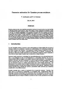
In this section we investigate the effect of the number of design points to the accuracy of estimating the model parameters. It is generally known that the likelihood function gets flatter as the number of design points decreases ( [3], §5.4). In two dimensions, this phenomenon manifests itself with the replacement of the peak that should appear in the vicinity of the correct parameter values, with a ridge that runs across the axis of one of the parameters. This is illustrated in Figure 1. For n = 20, the maximisation algorithm returned τ2 = 0.1 and τ2 = 0.08, which is the location of the main peak presented in the left panel of Figure 1. For n = 10, we can notice the ridge that exists at τ2 ∼ 3 and runs across the axis of τ1 . In this case the maximisation algorithm returned τ1 = −32 and τ2 = 3.4, which correspond to δ1 = 1.2 × 10⁷ and δ2 = 0.18. The interpretation of this solution is that when there are very few data available, the model can explain them with only one input, while the second is essentially rendered inactive, by setting its correlation length to an unrealistically high value. 70
5
0
50 Log Likelihood
Log Likelihood
60
40 30 20
−5
−10
10 0
−15
10
0 tau2
−10
0 tau1
10
10
(a) n = 20
0 tau2
−10
0 tau1
10
(b) n = 10
Figure 1: Log Likelihood (8) of data generated from a Gaussian process with τ = 0. For the left panel n = 20 design points were used and for the right n = 10. A question that then arises, is what is the minimum number of design points needed so as to avoid the above ‘degeneracy’. In our experiments the maximisation algorithm is initialised with the correlation lengths used for generating the data. We therefore make the assumption that if one of the estimated δ’s is above a certain threshold, then the respective output is rendered inactive, as a result of not having used sufficient design points. To obtain the minimum number of points needed for the model to explain the data using all the available inputs we drew samples from a Gaussian process for several combinations of inputs and design points. For each case, the experiment was run 1000 times, and we counted the number of realisations for which all the estimated δ’s were smaller than a threshold, which was set to 5. The results for an input δ of 1 are shown in table 1. The rows of this table correspond to the number of design points per input dimension (n/p) and the columns correspond to the number of input dimensions (p). The left part of the table shows the results for the REML method and the right for ML. Focusing on REML we see that for small dimensions using the rule of 10 point per input seems adequate for allowing all the runs to produce estimates within a reasonable range of δ. Using the same rule in 10 dimensions, almost 20% of the runs resulted in very large estimates for the correlation lengths. Examining the right part of table 1, which corresponds to the ML method, similar conclusions can be drawn. An important observation however, is that for the same number of design points and inputs, fewer runs resulted in estimates of δ within the predetermined range. This implies that 6
more design points might be generally needed for estimating the correlation lengths when using the ML method. We will attempt to explain this in section 3. Table 2 shows the same results when the correlation length used for generating the data was δ = 0.3. A striking difference is that for the same number of inputs, significantly more design points are needed for estimating the model parameters when the correlation between the observations is smaller. This is particularly evident for high dimensional inputs. Note also the different n/p ratios used in tables 1 and 2. n/p 5 10 15 20 25 30
p=2 93 100 100 100 100 100
p=3 81 100 100 100 100 100
REML p=5 p=8 46 42 99 92 100 99 100 100 100 100 100 100
p = 10 39 81 97 100 100 100
p=2 94 100 100 100 100 100
p=3 77 100 100 100 100 100
ML p=5 23 99 100 100 100 100
p=8 12 69 98 100 100 100
p = 10 11 39 88 99 100 100
Table 1: Percentage of realisations for which the estimated correlation lengths were less than 5. Input δ was 1. n/p 5 10 20 30 50
p=2 92 100 100 100 100
p=3 75 99 100 100 100
REML p=5 p=8 8 0 59 1 93 12 99 28 100 58
p = 10 0 0 0 1 7
p=2 82 100 100 100 100
p=3 57 95 100 100 100
ML p=5 6 38 89 99 100
p=8 0 0 2 17 50
p = 10 0 0 0 1 6
Table 2: Percentage of realisations for which the estimated correlation lengths were less than 5. Input δ was 0.3.
2.1
Evaluation using the Mahalanobis distance
In this section we investigate the effect of the number of design points on parameter estimation using the Mahalanobis distance. The Mahalanobis distance for both ML and REML methods follows a Chi squared distribution with np degrees of freedom, where np is the number of points used for prediction. In our experiments p we used np = n/2. The above Chi Squared distribution has mean ¯ the average Mahalanobis distance from the np and standard deviation 2np . If we denote by M successful runs out of 100, we define the normalised Mahalanobis distance as Mn =
¯ − np M p 2 2np
(23)
The normalised version of the Mahalanobis distance has the benefit of being independent from the number of evaluation points used, and when its absolute value is less than one, then the mean
7
n/p 10 15 20 25 30
p=2 1.50 0.73 0.38 0.37 0.27
p=3 1.86 0.97 0.62 0.58 0.43
REML p=5 2.72 1.62 1.21 0.97 0.69
p=8 2.07 1.42 1.15 0.92 0.84
p = 10 1.93 1.43 1.20 1.01 0.87
p=2 3.53 1.70 0.89 0.75 0.58
p=3 1.84 1.58 1.37 1.24 1.00
ML p=5 2.04 1.21 1.01 0.88 0.71
p=8 2.93 1.98 1.48 1.20 1.03
p = 10 3.16 2.29 1.84 1.45 1.27
Table 3: Normalised Mahalanobis distance Mn for different number of inputs and design points.
Mahalanobis distance is within a standard deviation from the theoretical mean. The normalised Mahalanobis distances for the data drawn in the previous section using δ = 1 are shown in table 3. Examining the results for REML, we see that for two to three inputs, 15 design points per input seem sufficient for obtaining an average Mahalanobis distance that is closer to the theoretical mean than 1 standard deviation. For 5-10 inputs 25-30 points per input are needed for getting the same result. Also the increasing trend indicates that for more than 10 inputs, more points per input will be needed for keeping the average Mahalanobis distance close to its theoretical mean. The respective results for ML, show that the distances are larger in average compared to those of REML. This may be an indication that the predictions made using ML might be slightly more overconfident compared to REML1 .
2.2
Conclusion
As a conclusion we can say that the estimation of hyperparameters depends both on the dimensionality of the input but also on the inherent correlation length of the data. We saw that for δ = 1, which represents a fairly smooth function, ten to 15 points per input suffice for 2-3 inputs, while for 5-10 inputs 25 to 30 points per input are needed. This number goes up dramatically as the output data vary faster. For example, we found that for 5 dimensions and δ = 0.3, 50 points per input are needed (i.e. n = 250), and this number increases steeply as more dimensions are added.
3
Comparison between ML and REML
In this section we highlight the main differences between the ML and REML estimation methods. We also try to provide some insight by individually examining their terms. Table 4 shows the average estimates of δ from the data used to make table 1. Table 5 shows the respective confidence intervals. The two tables show that ML slightly underestimates the correlation lengths and REML slightly overestimates them. However, the difference from the real value, which is δ = 1, is so small that it would probably have no effect on the prediction. The difference between the ML and REML estimates of δ seems to be consistent, as it is illustrated 1 We should note here that the primary use of the Mahalanobis distance is not to compare alternative models, but rather to indicate potential conflicts between the emulator and the simulator. However, because we are averaging the distances over many realisations, we believe that table 3 gives an indication of the comparative performance of ML and REML.
8
n/p 10 15 20 25 30
p=2 1.03 1.02 1.02 1.02 1.02
REML p=5 1.09 1.03 1.02 1.01 1.00
p=3 1.05 1.02 1.01 1.01 1.01
p=8 1.07 1.03 1.02 1.01 1.01
p = 10 1.07 1.03 1.02 1.01 1.01
p=2 0.93 0.99 1.00 1.00 1.01
p=3 0.92 0.96 0.97 0.99 0.99
ML p=5 0.89 0.94 0.96 0.97 0.98
p=8 0.99 0.98 0.98 0.98 0.98
p = 10 1.04 1.00 1.00 1.00 0.99
Table 4: Average estimates of δ as a function of the design points and the dimensionality of the input. n/p 10 15 20 25 30
p=2 0.011 0.008 0.006 0.005 0.005
REML p=5 0.018 0.010 0.007 0.006 0.005
p=3 0.013 0.007 0.005 0.005 0.004
p=8 0.023 0.013 0.010 0.008 0.007
p = 10 0.026 0.016 0.011 0.009 0.008
p=2 0.010 0.007 0.006 0.005 0.005
p=3 0.011 0.007 0.005 0.005 0.004
ML p=5 0.014 0.009 0.007 0.006 0.005
p=8 0.028 0.014 0.010 0.008 0.007
p = 10 0.047 0.019 0.012 0.009 0.008
Table 5: Confidence intervals (95%) for table 4.
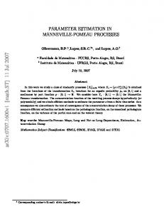
in figure 2. This figure shows the ML estimates plotted against those of REML, for p = 3. The REML estimates seem to always be higher than the ML, as it is indicated from the boundary that seems to exist along the line δML = δRL .
1.2
δ RL
1.1 1 0.9 0.8 0.7 0.7
0.8
0.9
1 δ ML
1.1
1.2
1.3
Figure 2: Scatter plot of δˆML against δˆRL , showing that δˆRL > δˆML . Section 2 highlighted two more differences between ML and REML: the first was that ML needed slightly more design points so as to explain the data using all the available inputs; the second was that the average Mahalanobis distance showed that ML might be slightly more overconfident than REML in its predictions. Finally, REML has the theoretical property of producing unbiased estimates of σ 2 , which was confirmed during our simulations. The following analysis will attempt to explain the above differences between REML and ML. The expressions that need to be maximised for estimating δ using the ML and REML methods (6, 9
10) can be written as 1 n LML ∝ − ln |A| − ln S 2 2 n−q 1 1 ln S − ln |H T A−1 H| LRL ∝ − ln |A| − 2 2 2
(24) (25)
ˆ T A−1 (y − H β) ˆ being the generalised residual sum of squares. For convenience with S ≡ (y − H β) we denote the terms involved in the above expressions as
1 L1ML ≡ − ln |A| 2 n L2ML ≡ − ln S 2
1 L1RL ≡ − ln |A| 2 n−q 2 LRL ≡ − ln S 2 1 L3RL ≡ − ln |H T A−1 H| 2
The terms L1ML and L1RL are identical and L2ML and L2RL differ only in their multiplying factors. To illustrate the function of the above terms within the expressions of the respective log likelihoods we use 5 data points drawn from a Gaussian Process in [0, 1] with δ = 1 and plot the above terms as a function of ln δ. The term L1ML (fig. 3 left panel) is known as the model complexity penalty ( [3], §5.4). This term favours larger correlation lengths because the model gets more rigid and therefore less complex. The right panel of figure 3 shows the data fit terms L2 , which are the only ones that depend on the data. The L2 terms support smaller correlation lengths because the model then gets more flexible and fits the data better. The compromise between these two terms gives the ML solution. 30
10
25
5
20
0 −5 L2
L1
15
−10
10 −15
5
−20
0 −5 −10
−25
−5
0 ln(δ)
5
−30 −10
10
(a) L1
−5
0 ln(δ)
5
10
(b) L2
Figure 3: The left panel shows he model complexity penalty L1 . The right panel shows the data fit terms L2ML (cont. line), L2RL (dashed line).
Figure 3 also provides a clue as to why the REML estimates of δ tend to be higher than those of ML. L2RL is bounded by L2ML and as a result has a less steep slope. This is likely to be the reason why the correlation lengths estimated with REML are generally higher than those estimated with ML. The left panel of figure 4 shows the L3RL term. The right panel of the same figure shows LML (continuous line), LRL (dashed line) and the difference LRL -L3RL (dashed red line). This figure indicates that the L3RL term helps equalising the two ‘wings’ (plateaus towards ±∞) of LRL . Perhaps 10
most importantly it helps eradicating the positive slope that appears in LML for ln δ ∈ [3, 8]. We can envisage a situation in which if the maximisation algorithm landed in the above interval, it would diverge towards +∞ for ML, while it would converge to the maximum of LRL . This could be a reason why REML explains the data using all the inputs more often than ML does. 1
10
0
8 6
−1
4 2
−3
L
L3
−2
0 −4
−2
−5
−4
−6 −7 −10
−6 −5
0 ln(δ)
5
−8 −10
10
(a) L3RL
−5
0 ln(δ)
5
10
(b) n = 10
Figure 4: L3RL is shown in the left panel. The right panel shows the LML and LRL terms (continuous and dashed black lines) and the difference LRL − L3RL (red dashed line). Finally, the lower Mahalanobis distances for REML, which indicate that is less overconfident than ML, might be due to the fact that REML accounts for the uncertainty in β and as a result, its predictions have greater variance. For the same reason we would expect the Mahalanobis distance for the Toolkit method to be even lower.
4
Accounting for the uncertainty in δ
In section 1 we saw that the REML and Toolkit methods for parameter estimation are derived from Maximum Likelihood by accounting for the uncertainty in β and σ 2 respectively. An obvious extension would be to account for our uncertainty about the value of δ. However, this is not as R straightforward as it is with the two other parameters, because the integral p(y|δ)p(δ) dδ can not be calculated analytically. We therefore have to resort to numerical or approximation methods. Two such methods are considered here: integration via MCMC and the normal approximation of the posterior distribution. Before using MCMC integration, there is one technicality that we need to address. The likelihood functions 3, 8 and 13 do not decay to zero as τ tends to ±∞; as a result, the posterior calculated using uniform priors is improper. This result is also proved in [4]. MCMC integration can fail to converge when improper posteriors are used. This problem can be alleviated using priors that make the posterior distribution proper, but at the same time will not alter drastically the shape of the likelihood, at least in the parameter range we are interested in. Two such priors are examined in the next section.
11
4.1 4.1.1
Correlation length priors Reference prior
The reference priors were proposed by Berger et al. [4] for 1 dimension, and were extended to higher dimensions by Paulo [5]. They can be considered as Jeffrey’s priors on the marginalised likelihood p(y|σ 2 , δ) and their derivation is based on the maximisation of the Kullback Leibler divergence between the prior and the posterior distribution. The reference prior is given by 1/2
p(τ ) ∝ |I(τ )| where
n-q
I= and Wk =
trW1 trW12
trW1 trW1 W2 .. .
··· ··· ···
(26)
trWp trW1 Wp .. .
trWp2 ∂A −1 A (I − H(H 0 A−1 H)−1 H 0 A−1 ) ∂τk
Figure 5 shows the logarithms of the likelihood, the reference prior and the resulting posterior distribution, for 10 points drawn from a 1 dimensional Gaussian process in [0, 1] with τ = 0. The reference prior is relatively flat in the region of interest, while it drops off as τ takes very large or very small values, hence making the posterior distribution proper. 60 40
Log Probability
20 0 −20 −40 −60 −80 −10
−5
0 tau
5
10
Figure 5: Log of the likelihood (dashed) reference prior (dotted) and posterior (continuous) distributions corresponding to 10 points drawn from a 1 dimensional GP in [0, 1] with τ = 0.
To check the effect of the reference prior on the estimates of δ we compared the REML estimates (δˆRL ) with the MAP estimates of the posterior formulated by the REML likelihood and the reference prior (δˆRF ). One hundred realisations of data drawn from a GP in [0, 1] were made for three different cases: a) p = 1, n = 10, δ = 1, b) p = 1, n = 10, δ = 0.3 and c) p = 3, n = 30, δ = 1. Figure 6 shows the histograms of the differences (δRL − δRF ). The majority of the errors is less than 0.02, which is expected to have a rather negligible effect in prediction.
12
35
50
30
40 30 20
60
25 20 15 10
10 0 −0.02
80
Occurences
Occurences
Occurences
60
40
20
5 0
0.02 0.04 Error
0.06
0 −0.01
0.08
(a)
−0.005
0 Error
0.005
0.01
0 −0.04
(b)
−0.02
0
0.02 Error
0.04
0.06
(c)
Figure 6: Histograms of the difference between the REML estimate δˆRL and the estimate obtained with the reference prior δˆRF for three cases a) p = 1, n = 10, δ = 1, b) p = 1, n = 10, δ = 0.3 and c) p = 3, n = 30, δ = 1.
4.1.2
Exponential Inverse Gamma prior
Apart from the reference prior we introduce here another prior that is derived from an exponential transformation g(x) = e−x of the inverse Gamma distribution. That is, if a random variable x follows an Exponential Inverse Gamma (EIG) distribution, then e−x will follow the inverse Gamma. The formula for the EIG distribution2 is � p(τ ) = e−ατ exp −γe−τ (27) The logarithm of the EIG distribution is shown in figure 7. The hyperparameter γ controls the the slope for τ → −∞ and α controls the slope for τ → ∞. The mode of this distribution is found at τ = − ln (α/γ). 60 40
Log Probability
20 0 −20 −40 −60 −80 −10
−5
0 tau
5
10
Figure 7: Logarithm of the EIG prior for α = 0.2667 and γ = 0.0595. This is clearly an informative prior, whose shape does not depend on the data as the shape of the reference prior does. As we are mainly interested in making the posterior distribution proper, we only wish to provide vague information on the value of δ. We start from the assumption that correlation lengths outside the range δ ∈ [0.05, 2] are very unlikely to occur. In the space of τ this translates to τ ∈ [−1.5, 6]. We place the mode of our prior at τ = −1.5. This implies the condition τ0 = − ln (α/γ) = −1.5. At τ1 = 6 we want the logarithm of our prior to have dropped by approximately 2, which represents a rough 95% interval. As the rate of this drop is determined 2 This
distribution is closely related to the Extreme Value Distribution
13
by the e−ατ term, we require that e−α(τ0 −τ1 ) = e2 . The above two conditions yield α = 0.2667 and γ = 0.0595. These values of the hyperparameters were used for the prior shown in figure 7. Figure 8 shows the likelihood also shown in figure 5, the EIG prior and the resulting posterior distribution. 60 40
Log Probability
20 0 −20 −40 −60 −80 −10
−5
0 tau
5
10
Figure 8: Log of the likelihood (dashed) EIG prior (dotted) and posterior (continuous) distributions corresponding to 10 points drawn from a 1 dimensional GP in [0, 1] with τ = 0.
To evaluate the effect of this prior on the estimates of δ we performed the same experiment as with the reference prior, and the results are shown in figure 9. The errors are comparable to those of the reference prior, although there is a small negative bias, which implies that that δ’s are slightly overestimated when the EIG prior is used. Nevertheless, the errors are rather small so we should not expect them to have a notable impact on prediction. On the other hand, the EIG priors are a lot cheaper computationally, which can be an important advantage in MCMC simulations.
60 40
Occurences
Occurences
Occurences
50
80
80
60 40 20
20 0 −0.08
60
100
100
−0.06
−0.04 −0.02 Error
(a)
0
0.02
40 30 20 10
0 −0.01 −0.008 −0.006 −0.004 −0.002 Error
(b)
0
0 −0.1
−0.08
−0.06 −0.04 Error
−0.02
0
(c)
Figure 9: Histograms of the difference between the REML estimate δˆRL and the estimate obtained with the EIG prior δˆEG for three cases a) p = 1, n = 10, δ = 1, b) p = 1, n = 10, δ = 0.3 and c) p = 3, n = 30, δ = 1.
Another advantage of using either of the above priors is that they might make the optimisation procedure for finding the ML estimates of δ more robust. The reason is that because the priors are essentially applying weight in the more interesting ranges of τ , the optimisation algorithm is less likely to converge to unrealistically large of small values for the correlation lengths.
14
4.2
Methods for accounting for the uncertainty in δ
As we mentioned at the beginning of this section, accounting for the uncertainty in δ is not possible via an analytic integration of p(η(x)|δ, y) w.r.t. δ. We now present two methods of sidestepping this problem.
4.2.1
MCMC integration
The first method involves the construction of an MCMC algorithm that can sample from the posterior p(τ |y). The resulting samples of τ can then be used for prediction. An outline of how this can be achieved is given below. We first estimate the value of τ that maximises p(τ |y) and call it τˆ. We then find the Hessian matrix at τˆ, using the expressions for the derivatives from equations (20 - 22). If we call this matrix Hτˆ we can then define a matrix Vτˆ = −Hτˆ−1 . We then setup the following MCMC (Metropolis) algorithm 1. Set τ (1) equal to τˆ 2. Add to τ (i) a normal variate drawn from N (0, Vτˆ ), call the result τ ∗ 3. Calculate the ratio α =
p(y|τ ∗ ) p(y|τ (i) )
4. Set τ (i+1) = τ ∗ with probability α and τ (i+1) = τ (i) with probability 1 − α 5. Repeat steps 2-4 until a sufficient number of samples has been drawn. Once a sufficient number of samples M has been drawn, we can do inference about the output of the emulator. For example, an estimate of the mean of η(x) can be ηˆ(x) =
M Z 1 X η(x)p(η(x)|τ (i) , y)dη M i=1
The main drawback of the MCMC based scheme, is that it is computationally demanding. It is reported however to give good coverage probability [2, 5].
4.2.2
Normal approximation of the posterior
An alternative method of obtaining samples of δ involves the approximation of the posterior p(τ |y) using a normal distribution, as described in [2]. As with MCMC, the mode τˆ of the posterior p(τ |y) is first found. Then the inverse Hessian matrix Vτˆ = −Hτˆ−1 is calculated. Finally, the posterior p(τ |y) is approximated with the normal distribution N (ˆ τ , Vτˆ ), which is used for drawing samples of τ . A benefit of this approach is that the samples are i.i.d., and is also significantly significantly faster than the MCMC based method. A potential problem however, can be that the samples are not drawn from the actual posterior, but from an approximation that may or may not be accurate. For example, if the optimisation procedure used for finding the mode τˆ converges to a local minimum, this mode will then be approximated but not the main one. Nevertheless, Nagy et al. [2] report coverage probabilities similar to those obtained with MCMC. 15
5
Conclusion
In this report we saw how three parameter estimation methods, ML REML and the Toolkit approach, are connected, via marginalisation of their likelihood functions. We also showed that the Toolkit approach is closely related to REML and that for n − p >> they become identical. We also derived expressions for the derivatives for the REML/Toolkit cost functions, which speed up significantly the optimisation process and are helpful when accounting for our uncertainty in δ. We then investigated the effect of the number of design points to the estimation of the correlation lengths. We saw that the accuracy of estimation strongly depends on the dimensionality of the input as well as on the inherent correlation length of the data. A main finding was that for moderately smooth data 15 points per dimension were needed for 2-3 dimensional inputs, while for 5-10 dimensions the estimates were satisfactory for 25-30 design points per input. It is also likely that more points per input will be needed for dimensions higher than 10. A comparison between the ML and REML methods, showed that the latter needed somewhat fewer design points for estimating the correlation lengths, while ML was slightly more overconfident in its prediction. This might as well be due to the fact that ML does not account for the uncertainty in β. Finally, we found that ML slightly underestimated and REML slightly overestimated the correlation lengths, but not by an amount that should have a notable effect on the predictions. In the final part of the report we considered two methods that account for the uncertainty in δ, one based on MCMC integration and one on the approximation of the posterior with a normal distribution. We focused on the application of priors that result in proper posterior distributions, as required by MCMC. We implemented the reference prior, and proposed a much simpler one, based on a transformation of the inverse gamma distribution. None of the priors seemed to alter the shape of the likelihood, in the parameter range of interest, but both priors resulted in proper posterior distributions. The evaluation of the normal approximation and the MCMC methods using the proposed priors consists work in progress.
References [1] D. Harville, “Bayesian inference for variance components using only error contrasts,” Biometrika, vol. 61, pp. 383–385, 1974. [2] B. Nagy, J. Loeppky, and W. Welch, “Correlation parameterization in random function models to improve normal approximation of the likelihood or posterior,” Dept. of Statistics, The University of British Columbia, URL http://stat.ubc.ca/Research/TechReports/techreports/229.pdf, Tech. Rep. 229, 2007. [3] C. E. Rasmussen and C. K. I. Williams, Gaussian Processes for Machine Learning (Adaptive Computation and Machine Learning). The MIT Press, December 2005. [4] J. O. Berger, V. D. Oliveira, and B. Sans´o, “Objective Bayesian analysis of spatially correlated data,” Journal of the American Statistical Association, vol. 96, no. 456, pp. 1361–1374, 2001. [5] R. Paulo, “Default priors for Gaussian processes,” Annals of Statistics, vol. 33, pp. 556–582, 2005.
16