Parameter Estimation for Optimal Object Recognition: Theory and

International Journal of Computer Vision, 21(3), 1{17 (1997)

c 1997 Kluwer Academic Publishers, Boston. Manufactured in The Netherlands.

Parameter Estimation for Optimal Object Recognition: Theory and Application 

STAN Z. LI

School of Electrical and Electronic Engineering Nanyang Technological University, Singapore 639798

Received February 2, 1994. Revised May 2, 1995.

Abstract.

Object recognition systems involve parameters such as thresholds, bounds and weights. These parameters have to be tuned before the system can perform successfully. A common practice is to choose such parameters manually on an ad hoc basis, which is a disadvantage. This paper presents a novel theory of parameter estimation for optimization-based object recognition where the optimal solution is de ned as the global minimum of an energy function. The theory is based on supervised learning from examples. Correctness and instability are established as criteria for evaluating the estimated parameters. A correct estimate enables the labeling implied in each exemplary con guration to be encoded in a unique global energy minimum. The instability is the ease with which the minimum is replaced by a non-exemplary con guration after a perturbation. The optimal estimate minimizes the instability. Algorithms are presented for computing correct and minimal-instability estimates. The theory is applied to the parameter estimation for MRF-based recognition and promising results are obtained.

Keywords: Learning from examples, Markov random elds, object recognition, optimization, parameter

estimation

1. Introduction Object recognition systems almost inevitably involve parameters such as thresholds, bounds and weights [17]. In optimization-based object recognition, where the optimal recognition solution is explicitly de ned as the global extreme of an objective function, these parameters can be part of the de nition of the objective function by which the global cost (or gain) of the solution is measured. The selection of the parameters is crucial for a system to perform successfully. Among all the admissible parameter estimates, only a subset of them lead to the desirable or correct solutions to the recognition. Among all the correct estimates, a smaller number of them are better in the sense that they lead to correct solutions for a larger variety of data sets. One of them may be optimal in the sense that it makes the vision procedure the most stable to uncertain

This work was supported by NTU project RG 43/95.

ties and the least prone to local optima in the search for the global optimum. The manual method performs parameter estimation in an ad hoc way by trial and error: A combination of parameters is selected to optimize the objective function, then the optimum is compared with the desirable result in the designer's perception and the selection is adjusted; this process is repeated until a satisfactory choice, which makes the optimum consistent with the desirable result, is found. This is a process of supervised learning from examples. When the objective function takes a right functional form, a correct manual selection may be made for a small number of data sets. However, there is no reason to believe that the manual selection is an optimal or even a good one. Such empirical methods have been criticized for its ad hoc nature. This paper aims to develop an automated, optimal approach for parameter estimation1 applied to optimization-based object recognition schemes.

2

Stan Z. Li

A theory of parameter estimation based on supervised learning is presented. The learning is \supervised" because exemplar is given. Each exemplary instance represents a desirable recognition result where a recognition result is a labeling of the scene in terms of the model objects. Correctness and optimality are proposed as the two-level criteria for evaluating parameter estimates. A correct selection of parameter enables the con guration given by each exemplary instance to be embedded as a unique global energy minimum. In other words, if the selection is incorrect, the exemplary con guration will not correspond to a global minimum. While a correct estimate can be learned from the exemplar, it is generally not the only correct solution. Instability is de ned as the measure of the ease with which the global minimum is replaced by a non-exemplar labeling after a perturbation to the input. The optimality minimizes the instability so as to maximize the ability to generalize the estimated parameters to other situations not directly represented by the exemplar. Combining the two criteria gives a constrained minimization problem: minimize the instability subject to the correctness. A non-parametric algorithm is presented for learning an estimate which is optimal as well as correct. It does not make any assumption about the distributions and is useful for cases where the size of training data obtained from the exemplar is small and where the underlying parametric models are not accurate. The estimate thus obtained is optimal with respect to the training data. The theory is applied to a speci c model of MRF recognition presented in [21]. The objective function in this model is the posterior energy of an MRF2 . The form of the energy function has been derived but it involves parameters that have to be estimated. The optimal recognition solution is the maximum a posteriori (MAP) con guration of an MRF. Experiments conducted show very promising results in which the optimal estimate serves well for recognizing other scenes and objects. Although automated and optimal parameter selection for object recognition in high level vision is an important and interesting problem which has been existing for a long time, reports on this topic are rare. Works have been done in related areas:

In [29] for recognizing 3D objects from dierent viewpoints, a function mapping any viewpoint to a standard view is learned from a set of perspective views. In [40], a network structure is introduced for automated learning to recognize 3D objects. In [30], a numerical graph representation for an object model is learned from features computed from training images. A recent work [28] proposes a procedure of learning compatibility coecients for relaxation labeling by minimizing a quadratic error function. Automated and optimal parameter estimation for low level problems has achieved signi cant progress. MRF parameter selection has been dealt with in statistics [2], [3] and in applications such as image restoration, reconstruction and texture analysis [8], [6], [10], [31], [42], [25]. The problem is also addressed from regularization viewpoint [37], [14], [33], [35]. The paper is organized as follows: Section 2 presents the theory. Section 3 applies the theory to an MRF recognition model. Section 4 presents the experimental results. Finally, conclusions are made in Section 5.

2. Theory of Parameter Estimation for Recognition In this section, correctness, instability and optimality are proposed for evaluating parameter estimates. Their relationships to non-parametric pattern recognition are discussed and non-parametric methods for computing correct and optimal estimates are presented. Prior to these, necessary notations for optimization-based object recognition are introduced. 2.1. Optimization-Based Object Recognition

In optimization-based recognition, the optimal solution is explicitly de ned as the extreme of an objective function. Let f be a con guration representing a recognition solution. The cost of f is measured by a global objective function E (f j ), also called the energy. The de nition of E is dependent on f and a number of K + 1 parameters  = [0 ; 1 ; : : : ; K ]T . As the optimality criterion for model-based recognition, it also relates to other factors such as the observation, denoted

Parameter Estimation for Optimal Object Recognition

G , and model references, denoted G 0 . Given G ; G 0

and , the energy maps a solution f to a real number by which the cost of the solution is evaluated. The optimal solution corresponds to the global energy minimum, expressed as: f  = arg min E (f j ) (1) f In this regard, it is important to formulate the energy function so that the \correct solution" is embedded as the global minimum. The energy may also serve as a guide to the search for a minimal solution. In this aspect, it is desirable that the energy should dierentiate the global minimum from other con gurations as much as possible. The energy function may be derived using one of the following probabilistic approaches: fully parametric, partially parametric and nonparametric. In the fully parametric approach, the energy function is derived from probability distributions in which all the involved parameters are known. Parameter estimation is a problem only in the partially parametric and the non-parametric cases. In the partially parametric case, the forms of distributions are given but some involved parameters are unknown. An example is the Gaussian distribution with an unknown variance and another is the Gibbs distribution with unknown clique potential parameters. In this case, the problem of estimating parameters in the objective function is related to estimating parameters in the related probability distributions. In the nonparametric approach, no assumptions are made about distributions and the form of the objective function is obtained based on experiences or pre-speci ed \basis functions" [29]. This also applies to situations where the data set is too small to have statistical signi cance. An important form for E in object recognition is the weighted sum of various terms, expressed as

E (f j ) = T U (f ) =

K X k=0

k Uk (f )

(2)

where U (f ) = [U0 (f ); U1 (f ); : : : ; UK (f )]T is a vector of potential functions. A potential function is dependent on f , G and G 0 , where the dependence can be nonlinear in f , and often measures the vi-

3

olation of a certain constraint incurred by the solution f . This linear combination of (nonlinear) potential functions is not an unusual form and can be found in matching and recognition works such as [11], [13], [9], [16], [18], [34], [27], [4], [41], [12], [26], [38], [39], [21]. Note that when E (f j ) takes the linear form, multiplying  by a positive factor  > 0 does not change the minimal con guration arg min E (f j ) = arg min E (f j ) (3) f f Because of this equivalent, an additional constraint should be imposed on  for the uniqueness. In this work,  is con ned to have a unit Euclidean length

kk =

v u K uX t

k=0

k2 = 1

(4)

Given an observation G , a model reference G 0 and the form of E (f j ), it is the  value that completely speci es the energy function E (f j ) and thereby de nes the minimal solution f . It is desirable to learn the parameters from exemplars so that the minimization-based recognition is performed in a right way. The criteria for this purpose are established in the next subsection. 2.2. Criteria for Parameter Estimation

An exemplary instance is speci ed by a triple (f; G ; G 0 ) where f is the exemplary con guration (recognition solution) telling how the scene (G ) should be labeled or interpreted in terms of the model reference (G 0 ). The con guration f may be a structural mapping from G to G 0 . Assume that there are L model objects; then at least L exemplary instances have to be used for learning to recognize the L object. Let the instances be given as f(f` ; G ` ; G 0` ) j ` = 1; : : : ; Lg (5) We propose two-level criteria for learning  from examples: 1. Correctness. This de nes a parameter estimate which encodes constraints into the energy function in a correct way. A correct estimate, denoted correct, should embed each f`

4

Stan Z. Li

into the minimum of the corresponding energy E (f ` j correct), that is f` = arg min E ` (f j correct) 8` (6) f

where the de nition of E ` (f j ) is dependent upon the given scene G ` and the model G 0` of a particular exemplary instance (f` ; G ` ; G 0` ) as well as . Brie y speaking, a correct  is one which makes the minimal con guration f  de ned in (1) coincide with the exemplary con guration f` . 2. Optimality. This is aimed to maximize the generalizability of the parameter estimate to other situations. A measure of instability is de ned for the optimality and is to be minimized. The correctness criterion is necessary for a vision system to perform correctly and is of fundamental importance. Only when this is met does the MRF model make a correct use of the constraints. The optimality criterion is not necessary in this regard but makes the estimate most generalizable.

Correctness In (6), a correct estimate correct enables the f to be encoded as the global energy minimum for this particular pair (G ; G 0 ). Therefore, it makes any energy change due to a con guration change from f to f 6= f positive, that is,
E ` (f j ) = E ` (f j ) ? E ` (f` j ) X = k [Uk (f ) ? Uk (f`)] (7) > 0

k

8f 2 F `

where

F ` = ff

j f 6= f` g

(8)

is the set of all non-f` con gurations. Let correct = f j
E ` (f j ) > 0; 8f 2 F ` ; 8`g (9) be the set of all correct estimates. The set, if nonempty, usually comprises not just a single point but a region in the allowable parameter space. Some of the points in the region are better in the sense of stability to be de ned below.

Instability The value of the energy change
E ` (f j ) > 0 can be used to measure the (local) stability of  2 correct with respect to a certain con guration f 2 F ` . Ideally, we want E ` (f` j ) to be very low and E ` (f j ) to be very high, such that
E ` (f j ) is very large, for all f 6= f` . In such a situation, f` is expected to be a stable minimum where the stability is said w.r.t. perturbations in the observation and w.r.t. the local minimum problem with the minimization algorithm. The smaller is
E ` (f j ), the larger is the chance with which a perturbation to the observation will cause
E ` (f j correct) to become negative to violate the correctness. When
E ` (f j correct) < 0, f` no longer corresponds to the global minimum. Moreover, we assume that con gurations f whose energies are slightly higher than E ` (f` j ) are possibly local energy minima at which an energy minimization algorithm is most likely to get stuck. Therefore, the energy dierence, i.e. the local stabilities should be enlarged. One may de ne the global stability as the sum of all
E ` (f j ). For reasons to be explained later, instability, instead of stability, is used for evaluating . The local instability for a correct estimate  2 correct is de ned as (10) c` (; f ) =
E ` (1f j ) where f 2 F ` . It is \local" because it considers only one f 2 F ` It is desirable to choose  such that the value of c` (; f ) is small for all f 2 F `. Therefore, we de ned the following global p-instability of  8 1 exemplar instances, X = fx` (f ) = U ` (f ) ? U `(f` ) j f 2 F ` ; 8`g (19) contains training data from all the instances. X is the K + 1 dimensional data space in which x's are points. The correctness (7) can be written as T x(f ) > 0 8x 2 X (20) In pattern recognition, T x is called a linear classi cation function when considered as a function of x; T x(f ) is called a generalized linear classi cation function when considered as a function of f . There exist useful theories and algorithms for linear pattern classi cation functions [11]. Equation T x = 0 is a hyperplane in the space X , passing through the origin x(f) = 0. With a correct , the hyperplane divides the space into two parts, with all x(f ) (f 2 F ) in one side, more exactly the \positive" side, of the hyperplane. The Euclidean distance from x to the hyperplane is equal to T x=kk, a signed quantity. After the normalization (4), the point-tohyperplane distance is just T x(f ). The correctness can be judged by checking the minimal distance from the point set X to the

6

Stan Z. Li x2

x2

T

w x >0

x"

x"’ x’

(2)

L

x’ x"

x1

x1 o

o

(1)

L wTx < 0

(1)

L

(2)

(3)

L

(3)

L

L

Fig. 1. Correct and incorrect parameter estimates. A case where the C1 -optimal hyperplane is parallel to x0 x00 .

hyperplane. We de ne the \separability" as the smallest distance value

S () = min T x(f )=kk f

(21)

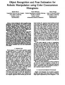
The above can also be considered as the stability of the system with a given . The correctness is equivalent to the positivity of the separability. It is helpful to visually illustrate the optimality using C1 . With C1 , the minimal-instability solution is the same as the following minimax solution  = arg 2min C1 () = correct   (22)
E ( f j  ) arg 2min max f 2F correct

In this case, S () = 1=C1 () and the above is maximal-separability. Fig.1 qualitatively illustrates correct/incorrect and the maximal-separability parameters. It is an example in two dimensional space where an energy change takes the form of
E (f j ) = T x(f ) = 1 x1 + 2 x2 . The point x(f) = 0 coincides with the origin of the x1 {x2 space. Data x(f ) (f 2 F ) are shown in lled dots. The three lines L(1), L(2) and L(3) represent three hyperplanes, corresponding to three dierent estimates of parameters . Parameter estimates for L(1) and L(2) are correct

Fig. 2. A case where the optimal hyperplane is perpendicular to ox0 .

ones because they make all the data points in the positive side of the hyperplane and thus satisfy Eq.(7). However, L(3) is not a correct one. Of the two correct estimates in Fig.1, the one corresponding to L(1) is better than the others in terms of C1 . The separability determines the range of disturbances in x within which the exemplary con guration f remains minimal. Refer to point x0 = x(f 0 ) in the gure. Its distance to L(2) is the smallest. The point may easily deviate across L(2) to the negative half space due to some perturbation in the observation d. When this happens,
E (f j ) < 0, causing E (f 0 j ) to be lower than E (f j ). This means that f is no longer the energy minimum. If the parameters are chosen as those corresponding to L(1) , the separability is larger and the violation of the correctness is less likely to happen. The dashed polygon in the gure forms the convex hull (polytope) of the data set. Only those data points which form the hull aect the minimax solution whereas those inside the hull are ineective. The ineective data points inside the hull can be removed and only the eective points, the number of which may be small compared to the whole data set, need be considered in the solution nding process. This increases the eciency. There are two possibilities for the orientation of the maximal-separability hyperplane with respect

Parameter Estimation for Optimal Object Recognition

Algorithm learning(, X ) /* Learning correct and optimal  */ Begin Algorithm initialize(); do f last ; if (T x > 0 9x 2 X ) f correct();  =kk; g

P

 ?  +  x2X (Txx)3 ;  =kk; T ? k < ); g until (klast  return( = );

End Algorithm

Fig. 3. Algorithm for nding the optimal combination of parameters.

to the polytope. The rst is that the optimal hyperplane is parallel to one of the sides (faces in cases of 3D or higher dimension parameter space) of the polytope, which is the case in Fig.1. The other is that the optimal hyperplane is perpendicular to the line linking the origin  and the nearest data point, which is the case in Fig.2. This is a property we may use to nd the minimax solution. When the points constituting the polytope are identi ed, all the possible solutions can be enumerated; when there are only a small number of them, we can nd the minimax solution by an exhaustive comparison. In Fig.2, L(2) is parallel to x0 x00 , and L(3) is parallel to x0 x000 but L(1) is perpendicular to 0x0 . Let 1 , 2 and 3 be the sets of parameters corresponding to L(1), L(2) and L(3). Suppose in the gure, the following relations hold: S (1 ) > S (2 ) and S (1 ) > S (3 ); then 1 is the best estimate because it maximizes the separability. The minimax solution (22) with p = 1 was used in the above only for illustration. With p = 1, a continuous change in x may lead to a discontinuous change in the C1 -optimal solution. This is due to the decision-making nature of the de nition which may cause discontinuous changes in the minimum. Other p-instability de nitions,

7

with p = 1 or 2 for example, are used in our practice because they give more stable estimates. 2.4. A Non-parametric Learning Algorithm

Consider the case when p = 2. Because T x  0, minimizing C2 () is equivalent to minimizing its square X 1 [C2 ()]2 = (23) T 2 x2X ( x) The problem is given formally as P 1 minimize x2X (T x)2 subject to kk = 1 T x > 0 8x 2 X

(24)

This is a nonlinear programming problem and can be solved using the standard techniques. In this work, a gradient-based, non-parametric algorithm is used to obtain a numerical solution. The perceptron algorithm [32] has already provided a solution for learning a correct parameter estimate. It iterates on  to increase the objective of the form T x based on the gradient information where the gradient is simply x. In one cycle, all x 2 X are tried in turn to adjust . If T x > 0, meaning x is correctly classi ed under , no action is taken. Otherwise if T x  0,  is adjusted according to the following gradient-ascent rule:

 ?  + x

(25)

where  is a small constant. The updating is followed by a normalization operation

 =kk (26) when kk = 1 is required. The cycle is repeated

until a correct classi cation is made for all the data and thus a correct  is learned. With the assumption that the solution exists, also meaning that the data set X is linearly separable from the origin of the data space, the algorithm is guaranteed to converge after a nite number of iterations [11]. P The objective function [C2 ()]2 = x2X (T1x)2 can be minimized in a similar way. The gradient is

8

Stan Z. Li

r[C2 ()]2 = ?2

X

x

T 3 x2X ( x)

(27)

X for generalization to other data. Better results

(28)

2.5. Reducing Search Space

An updating goes as follows

 ?+

X

x2X

x

(T x)3

where  is a small constant. If  were unconstrained, the above might diverge when (T x)3 becomes too small. However, the updating is again followed by the normalization kk = 1. This process repeats until  converges to . In our implementation, the two stages are combined into one procedure as shown in Fig.3. In the procedure, initialize() sets  at random, T ? correct() learns a correct  from X and (klast k < ), where  > 0 is a small number, veri es the convergence. The algorithm is very stable. The amount of change in each minimization itP eration is  x2X (Txx)3 . The in uence from x is weighted by 1=(T x)3 . This means that those x with smaller T x values (closer to the hyperplane) have bigger force in pushing the hyperplane away from themselves; whereas those with big T x values (far away from the hyperplane) have small in uence. This eectively stabilizes the learning process. When p = 1, we are facing the minimax problem (22). An algorithm for solving this is the \Generalized Portrait Technique" [36] which is designed for constructing hyperplanes with maximum separability. It is extended by Boser et al. [5] to train classi ers of the form T (x) where (x) is a vector of functions of x. The key idea is to transform the problem into the dual space by means of the Lagrangian. This gives a quadratic optimization with constraints. The optimal parameter estimate is expressed as a linear combination of supporting patterns where the supporting patterns correspond to the data points nearest to the hyperplane. Two bene ts are gained from this method: there are no local minima in the quadratic optimization and the obtained maximum separability is insensitive to small changes of the learned parameters. The  computed using the non-parametric procedure is optimal with respect to the training data X . It is the best result that can be obtained from

may be obtained, provided that more knowledge about the training data is available.

The data set X in (19) may be very large because there are a combinatorial number of possible con gurations in F = ff 6= fg. In principle, all f 6= f should be considered. However, we assume that the con gurations which are neighboring f have the largest in uence on the selection of . De ne the neighborhood of f as Nf = ff = (f1 ; : : : ; fm ) j fi 6= fi ; fi 2 L; 91 i 2 Sg (29) where 91 reads \exists one and only one" and L is the set of admissible labels for every fi . The Nf consists of all f 2 F that dier from f by one and only one component. This con nement reduces the search space to an enormous extent. After the con guration space is con ned to Nf, the set of training data is computed as X = fx = U (f ) ? U (f) j f 2 Nfg (30) which is much smaller than the X in Eq.(19).

3. Application in MRF Object Recognition The theory is applied to the parameter estimation for MRF object recognition where the form of the energy is derived based on MRFs. MRF modeling provides one approach to optimization-based object recognition [24], [7], [1], [19], [21]. The MAP solution is usually sought. The posterior distribution of con gurations f is of the Gibbs form [2]

P (f j d) = Z ?1e?E(f j )

(31)

where Z is a normalizing constant called the partition function and E (f j ) is the posterior energy function measuring the global of f . In the following, E (f j ) is de ned and converted to the linear form T U (f ).

Parameter Estimation for Optimal Object Recognition 3.1. Posterior Energy

An object or a scene is represented by a set of features where the features are attributed by their properties and constrained to one another by contextual relations. Let a set of m features (sites) in the scene be indexed by S = f1; : : :; mg, a set of M features (labels) in the considered model object by L = f1; : : : ; M g, and everything in the scene not modeled by labels in L by f0g which is a virtual NULL label. The set union L+ = L [ f0g is the augmented label set. The structure of the scene is denoted by G = (S ; d) and that of the model object by G 0 = (L; D) where d denotes the visual constraints on features in S and D describes the visual constraints on features in L where the constraints can be e.g. properties and relations between features. Let object recognition be posed as assigning a label from L+ to each of the sites in S so as to satisfy the constraints. The labeling (con guration) of the sites is de ned by f = ff1 ; : : : ; fm g in which fi 2 L+ is the label assigned to i. A pair (i 2 S ; fi 2 L+ ) is a match or correspondence. Under contextual constraints, a con guration f can be interpreted as a mapping from the structure of the scene G = (S ; d) to the structure of the model object G 0 = (L; D). Therefore, such a mapping is denoted as a triple (f; G ; G 0 ). The observation d = (d1 ; d2 ), which is the features extracted from the image, consists of two sources of constraints, unary properties d1 for single-site features such as color and size, and binary relations d2 for pair-site features such as angle and distance. More speci cally, each site i 2 S(k)is associated with a set of K1 properties fd1 (i) j k = 1; : : : ; K1; i 2 Sg and each pair of sites with a set of K2 relations fd(2k) (i; i0 ) j k = 1; : : : ; K2; i; i0 2 Sg. In the model object library, we have model features fD1(k) (I ) j k = 1; : : : ; K1; I 2 Lg and fD2(k) (I; I 0 ) j k = 1; : : : ; K2 ; I; I 0 2 Lg (note that L excludes the NULL label). Under the labeling f , the observation d is assumed to be a noise contaminated version of the corresponding model features D as

d1 (i) = D1 (fi ) + e(i) d1 (i; i0 ) = D2 (fi ; fi0 ) + e(i; i0)

(32) (33)

9

where fi ; fi0 6= 0 are non-NULL matches and e is a white Gauss noise; that is, d1 (i) and d2 (i; i0 ) are white Gaussian distributions with conditional means D1 (fi ) and D2 (fi ; fi0 ), respectively. The posterior energy E (f ) = U (f j d) takes the form P P P E (f ) = i2S V1 (fi ) + i2S i0 2Ni V2 (fi ; fi0 )+ P V1 (d1 (i) j fi )+ Pi2S :fi 6=0 P 0 i2S :fi 6=0 i0 2S?fig:fi0 6=0 V2 (d2 (i; i ) j fi ; fi0 ) (34) The rst and second summations are due to the joint prior probability of the MRF labels f ; the third and fourth are due to the pdf of d conditional on f (also the likelihood of f for xed d), respectively. In all cases, an Ni of the neighborhood system N on S can consist of all the other sites i0 6= i. This is a trivial case for MRF. In RS matching, it can consist of all the other sites which are related to i by any relations in d. When the scene is very large, Ni includes only those of the other sites which are within a spatial distance from i Ni = fi0 2 S j [dist(featurei0 ; featurei )]2  ; i0 6= ig where dist(A; B ) denotes some distance between A and B and  is an integer. The distance function needs be de ned appropriately for non-point features. The single-site potential is de ned as  if fi = 0 V1 (fi ) = 0v10 otherwise (35) where v10 is a constant. If fi is the NULL label, it incurs a penalty of v10 ; or nil penalty otherwise. The pair-site potential is de ned as  if fi = 0 or fi0 = 0 V2 (fi ; fi0 ) = v020 otherwise (36) where v20 is a constant. If either fi or fi0 is the

NULL , it incurs a penalty of v20 or nil penalty

otherwise. The above clique potentials de ne the prior energy U (f ). The above prior potentials are de ned in a similar way to the prior which penalizes the line process [15], [23]. They may also be de ned in terms of stochastic geometry [1].

10

Stan Z. Li

When the noise e is independent, the likelihood potentials are V1 (d18 (i) j fi ) = PK1 (k) (k) (k) 2 2 > > k=1 [d1 (i) ? D1 (fi )] =2[1 ] < (37) if fi 6= 0 > 0 > : otherwise and V82 (d2 (i; i0 ) j fi ; fi0 ) = PK2 (k) 0 D(k) (f ; f 0 )]2 =2[(k) ]2 > > 2 2 i i k=1 [d2 (i; i ) ? < if i0 6= i&fi 6= 0 & fi0 6= 0 (38) > > :

0

otherwise

where [n(k) ]2 (k = 1; : : : ; Kn and n = 1; 2) are the variances of the corresponding noise components. The vectors D1 (fi ) and D2 (fi ; fi0 ) are the \mean vectors", conditioned on fi and fi0 , for the random vectors d1 (i) and d2 (i; i0 ), respectively, conditioned on the con guration f . The assumptions of the independent and Gaussian noise may not be accurate but oers an approximation when an accurate observation model is not available. It helps us derive the functional form of the objective function. 3.2. Energy in Linear Form

Parameters involved in E (f ) are the noise variances [n(k) ]2 and the prior penalties vn0 (n = 1; 2). Let the parameters be denoted uniformly by  = fn(k) j k = 0; : : : ; Kn; n = 1; 2g. For k = 0,

n(0) = vn0 and for k  1, n(k) = (2[n(k) ]2 )?1

(39) (40)

Note all n(k)  0. Let the dierent energy components be uniformly denoted by U = fUn(k) j k = 0; : : : ; Kn ; n = 1; 2g. For k = 0,

U1(0) (f ) = N1 = #ffi = 0 j i 2 Sg (41)

is the number of NULL labels in f and

U2(0)(f ) = N2 = (42) #ffi = 0 or fi0 = 0 j i 2 S ; i0 2 Ni g is the number of label pairs at least one of which is

NULL . For k  1, Un(k) (f ) relates to the likelihood

energy components; They measure how much the observations dn(k) deviate from the should-be true ( k ) values Dn under f : 4 U (k) (d j f ) = U1(k) (f ) X = 1 [d1(k) (i) ? D1(k) (fi )]2 =f2[1(k) ]2 g (43) i2S ;fi 6=0

and

4 U (k) (d j f ) = U2(k) (f ) = P P2

i2Sh;fi 6=0 i0 2S ;i0 6=i;fi0 6=0 i (44) 2 d2(k) (i; i0 ) ? D2(k) (fi ; fi0 )

After some manipulation, the energy can be written as

E (f j ) =

Kn 2 X X

n=1 k=0

n(k) Un(k) (f ) = T U (f ) (45)

where  and U (f ) are column vectors of K1 + K2 + 2 components. Given an instance (f; G ; G 0 ), the U (f) is a known vector of real numbers. The  is a vector of unknown weights to be found. The stability follows immediately as
E (f j ) = T x(f ) (46) where x(f ) = U (f ) ? U (f). Some remarks on , U (f ) and E are in order. Obviously, all n(k) and Un(k) are non-negative. In the ideal case of exact (possibly partial) matching, all Un(k) (f ) (k  1) are zeros because d1(k) (i) and D1(k) (fi ) are exactly the same and so are d2(k) (i; i0 ) and D2(k) (fi ; fi0 ). In the general case of inexact matching, the sum of the Un(k) should be as small as possible for the minimal solution. The following are some properties of E :  Given f , E (f j ) is linear in . Given , it is linear in U (f ).

Parameter Estimation for Optimal Object Recognition

 For  > 0,  and  are equivalent, as have been discussed.

V (d j fi ) =

 The values of n(0) relative to those of n(k) (k  1) aect the rate of NULL labels. The

higher the penalties n(0) are, the more sites in S will be assigned non-NULL labels; and vice versa. The rst property enables us to use the results we established on linear classi ers for learning correct and optimal . According to the second property, a larger n(k) relative to the rest makes the constraint d(nk) and Dn(k) play a more important role. Useless and mis-leading constraints d(nk) and Dn(k) should be weighted by 0. Using the third property, one can decrease n(0) values to increase the number of the NULL labels. This is because for the minimum energy matching, lower cost for NULL labels makes more sites be labeled NULL , which is equivalent to discarding more not-so-reliable nonNULL labels into the NULL bin. 3.3. How Minimal Con guration Changes

The following analysis examines how the minimal con guration f  = arg minf E (f j ) changes as the observation changes from d0 to d = d0 + d where d is a perturbation. In the beginning when kdk is close to 0, f  should remain as the minimum for a range of such small d. This is simply because E (f j ) is continuous with respect to d. When the perturbation becomes larger and larger, the minimum has to give way to another con guration. When should a change happens? To see the eect more clearly, assume the perturbation is in observation components relating to only a particular i so that the only changes are d0(1k) (i) ! d(1k) (i) and d0(2k) (i; i0 ) ! d(2k) (i; i0), 8i0 2 Ni . First, assume that fi is a non-NULL label (fi 6= 0) and consider such a perturbation d that incurs a larger likelihood potential. Obviously, as the likelihood potential (conditioned on ffi0 6= 0 j i0 2 Ni g)

11

1(k) (d(1k) (iP ) ? D1(k) (fi ))2 + K2 (k) i0 2S ;i0 6=i;fi0 6=0 k=1 2 (d(2k) (i; i0 ) ? D2(k) (fi ; fi0 ))2 PK1

Pk=1

(47)

increases, it will eventually become cheaper for fi 6= 0 to change to fi = 0. More accurately, this should happen when

V (d j fi ) > 1(0) +

X

i0 2Ni ;fi0 6=0

2(0) = 1(0) + N2i 2(0) (48)

where

N2i = #fi0 2 Ni j fi0 6= 0g

(49)

is the number of non-NULL labeled sites in Ni under f . Next, assume fi = 0 and consider such a perturbation that incurs a smaller likelihood potential. The perturbation has to be such a coincidence that d and D become more resemblant to each other. As the conditional likelihood potential

V (d j fi ) =

PK1

Pk=1

1(k) (d(1k) (iP ) ? D1(k) (fi ))2 +

K2 i0 2S ;i0 6=i;fi0 6=0 k=1 2(k) (d(2k) (i; i0 ) ? D2(k) (fi ; fi0 ))2

(50)

decreases, it will eventually become cheaper for

fi = 0 to change to one of the non-NULL labels, fi 6= 0. More accurately, this should happen when V (d j fi ) < 1(0) +

X

i0 2Ni ;fi0 6=0

2(0) = 1(0) + N2i 2(0) (51)

The above analysis shows how the minimal con guration f  adjusts as d changes when  is xed. On the other hand, the f  can be maintained unchanged by adjusting ; this means a dierent encoding of constraints into E .

12

Stan Z. Li

4. Experiments

of model patterns plus spurious lines as shown in Fig.5(b). The exemplary con guration f is shown in Fig.5(a). It maps the scene to one of the models given in Fig.4. The alignment between the dotted lines of the scene and the solid lines of the model gives the non-NULL labels of f whereas the unaligned lines of the scene are labeled as NULL . The following four types of bilateral relations are used (n = 2; K2 = 4): 0 0 (1) d(1) 2 (i; i ): the angle between lines i and i , (2) (2) d2 (i; i0 ): the distance between the midpoints of the lines, 0 (3) d(3) 2 (i; i ): the minimum distance between the end-points of the lines, and 0 (4) d(4) 2 (i; i ): the maximum distance between the end-points of the lines. Similarly, there are four model relations D2(k) (I; I 0 ) (k = 1; : : : ; 4) of the same types. No unary properties are used (K1 = 0). The G and G 0 are composed of these 4 relational measurements. Therefore, there are ve components (k = 0; 1; : : : ; 4) in x and . The C2 -optimal parameters are computed as  = f2(0) ; 2(1) ; : : : ; 2(4) g = f0.58692, 0.30538, 0.17532, 0.37189, 0.62708g which satis es kk = 1. The computation takes a few seconds on an HP series 9000/755 workstation. To be used for recogni-

The following experiments demonstrate: (i) the computation (learning) of the optimal parameter  from the exemplary instance given in the form of a triplet (f; G ; G 0 ), and (ii) the use of the learned estimate  to recognize other scenes and models. The non-parametric learning algorithm is used because the data size is too small to assume a signi cant distribution. The convergence of the learning algorithm is demonstrated. 4.1. Recognition of Line Patterns

This experiment performs the recognition of simulated objects of line patterns under 2D rotation and translation. There are six possible model objects shown in Fig.4. Fig.5 gives the exemplary instance used for parameter estimation. The scene is given in the dotted and dashed lines which are generated as follows: (1) Take a subset of lines from each of the three objects in Fig.4(a)-(c); (2) rotate and translate each of the subsets, respectively; (3) mix the transformed subsets ; (4) randomly deviate the position of the endpoints of the lines, which results in the dotted lines; and (5) add spurious lines, shown in the dashed lines. The the generated scene consists of several subsets 15 22

6 9

3

12 2324 20 18 4 13 19 27 21 5 14 2 28 3 11 16 25 78 26 17 1 b

2

6

1

1

10 17 13

78 9

8 7

22 19 21 24 20 23

12

43 6 1 5 9 2 e

11 Fig. 4.

11 6

4 7

2

9 8

10 14 12 13

c

15 16 18

3 4

3

14 1317 11

14

5

d

5

14 17 1 13 5 15 10 6 7 16 2 9 11 12 8

10

a

4

15 1012 16 17 13

7 8 2 10

14 11 f

18 21 28 1 27 3 25 6 26 29 30 4 23 22 5 12 2024 9 1519 16

Six objects of line patterns in the model base.

Parameter Estimation for Optimal Object Recognition

13

15 6 9

22

12 2324 20 18 4 13 19 27 21 5 14 2 28 3 11 16 25 78 26 17 1 10

a Fig. 5.

b

An exemplary instance consisting of (a) exemplary con guration f, (b) scene G and (c) model G 0 .

tion,  is multiplied by a factor of 0:7=2(0), yielding the nal weights  =f0.70000, 0.36422, 0.20910, 0.44354, 0.74789g (our recognition system requires (2(0) ) = 0:7). The  is used to de ne the energy for recognizing other objects and scenes. The recognition results are shown in Fig.6. There are two scenes, one in the upper row and the other in the lower row, composed the dotted and dashed lines. The one in the upper was the one used in the exemplar whereas the scene in the lower contains sub-parts of the three model objects in Fig.4(d)-(f). Each scene are matched against the six model objects. The optimally matched object lines are shown in solid lines aligned with the scenes. The objects in the scenes are correctly matched to the model objects.

Fig. 6.

c

4.2. Recognition of Curved Objects

This experiment deals with jigsaw objects under 2D rotation, translation and uniform scaling. There are eight model jigsaw objects shown in Fig.7. In this case of curved objects, the features of an object correspond to the corner points of its boundary. For both the scene and the models, the boundaries are extracted from the images using the canny detector followed by hysteresis and edge linking. Corners are detected after that. No unary relations are used (K1 = 0). Denoting the corners by p1 ; : : : ; pm , the following ve types of bilateral relations are used (n = 2; K2 = 5) based on a similarity-invariant curve representation of curves [20]:

a

b

c

d

e

f

The optimal parameter estimate learned from the exemplar is used to recognize other scenes and models (see text).

14

Stan Z. Li

Fig. 7.

Eight model jigsaw objects.

0 (1) d(1) i pi0 and 2 (i; i ): ratio of curve arc-length pd 0 chord-length pi pi , 0 (2) d(2) 2 (i; i ): ratio of curvature at pi and pi0 , (3) (3) d2 (i; i0 ): invariant coordinates vector, 0 (4) d(4) 2(5) (i; i ): invariant radius vector, and (5) d2 (i; i0 ): invariant angle vector They are computed using information about both the boundaries and the corners. Similarly, there are ve model relations D2(k) (I; I 0 ) (k = 1; : : : ; 5) of the same types. Therefore, there are six components (k = 1; : : : ; 5) in each x and , one for the NULL and ve for the above relational quantities.

a

Fig. 8.

Fig.8 gives the exemplary instance used for parameter estimation. The scene in Fig.8(b) contains rotated, translated and scaled parts of one of the model jigsaws given in Fig.7. Some objects in the scene are considerably occluded. The alignment between the model jigsaw (the highlighted curve in (a)) and the scene gives non-NULL labels of f whereas the un-aligned boundary corners of the scene are labeled as NULL . The C2 -optimal parameters are computed as  = f2(0) ; 2(1) ; : : : ; 2(6) g = f0.95540, 0.00034, 0.00000, 0.06045, 0.03057, 0.28743g which satis es

b

c

An exemplary instance consisting of (a) exemplary con guration f, (b) scene G and (c) model G 0 .

Parameter Estimation for Optimal Object Recognition

15

The learned estimate is used to recognize other scenes and models. The matched model jigsaw objects are aligned with the scene.

Fig. 9.

kk = 1. It takes a few seconds on the HP work-

0 station. Note that the weight 2(2) for d(2) 2 (i; i ) (2) and D2 (I; I 0 ) (ratio of curvature) is zero. This means that this type of feature is not reliable enough to be used. Because our recognition system has a xed value of 2(0) = 0:7,  is multiplied by a factor of 0:7=2(0), yielding the nal weights  =f0.70000, 0.00025, 0.00000, 0.04429, 0.02240, 0.21060g. The  is used to de ne the energy function for recognizing other objects and scenes. The recognition results are shown in Fig.9. There are two scenes, one in the left column and the other in right column. The scene on the left was the one used in the exemplar and on the right is a new scene. The optimally matched model objects are shown in the highlighted curves aligned

with the scenes. The same results can also be obtained using the C1 -optimal estimate which is f0.7, 0.00366, 0.00000, 0.09466, 0.00251g.

4.3. Convergence

The parameter estimation algorithm is very stable and has a nice convergence property. Fig.10 shows how the global instability measure C2 and one of the learned parameters 2(3) evolve given dierent starting points. The values become stabilized after hundreds of iterations and dierent starting points converge to the same point.

10

0.50

Parameter value

Global instability

0.40

1

0.30 0.20 0.10

0

1

10

100 Iterations

Fig. 10.

1000

0.00

1

10

100 Iterations

Convergence of the algorithm with dierent starting points. Left: trajectories of C2 . Right: trajectories of 2(3) .

1000

16

Stan Z. Li

References

5. Conclusion

While manual selection is a common practice in object recognition systems, this paper has presented a novel theory for automated, optimal parameter estimation in optimization-based object recognition. The theory is based on learning from examples. Mathematical principles of correctness and instability are established and de ned for the evaluation of parameter estimates. A learning algorithm is presented for computing the optimal, i.e. minimal-instability, estimate. An application to the MRF-based recognition is given. Experiments conducted show very promising results. Optimal estimates automatically learned from examples can well be generalized for recognizing other scenes and objects. The exemplary instances are given to re ect the designer's judgment of desirable solutions. However, a recognizer with a given functional form can not be trained by arbitrary exemplar. The exemplar should be selected properly to re ect the correct semantics, in other words, they should be consistent with the constraints with which the functional form is derived. Assuming the form of the objective function is right and the exemplar contains useful information, then the more exemplary instances are used to train, the more generalizable is the learned parameter estimate. The learning procedure also provides a means of checking the validity of the energy function derived from mathematical models. An improper mathematical model leads to an improper functional form. If no correct parameter estimates can be learned, it is a diagnostic symptom that the assumptions used in the model are not suitable for modeling the reality of the scene. The procedure also provides useful information for feature selection. Components of the optimal parameter estimate will be zero or near zero for instable features.

Notes 1. In this work, parameter \selection", \estimation" and \learning" are used interchangeably. 2. The interested reader is referred to [22] for a comprehensive reference in MRF modeling. 3. This is because for the p-norm de ned by y p = ( y1 p + y2 p + + yn p )1=p , we have limp!1 y p = maxj yj . k k

j

j

j

j

j

j






j

j

k k

1. Baddeley, A. J. and van Lieshout, M. N. M. (1992). \Object recognition using Markov spatial processes". In Proceedings of IEEE International Conference Pattern Recognition, volume B, pages 136{139. 2. Besag, J. (1974). \Spatial interaction and the statistical analysis of lattice systems" (with discussions). Journal of the Royal Statistical Society, Series B, 36:192{236. 3. Besag, J. (1975). \Statistical analysis of non-lattice data". The Statistician, 24(3):179{195. 4. Bhanu, B. and Faugeras, O. D. (1984). \Shape matching of two-dimensional objects". IEEE Transactions on Pattern Analysis and Machine Intelligence, 6(2):137{ 155. 5. Boser, B. E., Guyon, I. M., and Vapnik, V. N. (1992). \A training algorithm for optimal margin classi ers". In Proceedings of the Fifth Annual ACM Workshop on Computational Learning Theory, Pittsburgh, Pennsylvania. 6. Cohen, F. S. and Cooper, D. B. (1987). \Simple parallel hierarchical and relaxation algorithms for segmenting noncasual Markovian random elds". IEEE Transactions on Pattern Analysis and Machine Intelligence, 9(2):195{218. 7. Cooper, P. R. (1990). \Parallel structure recognition with uncertainty: Coupled segmentation and matching". In Proceedings of IEEE International Conference on Computer Vision, pages 287{290. 8. Cross, G. C. and Jain, A. K. (1983). \Markov random eld texture models". IEEE Transactions on Pattern Analysis and Machine Intelligence, 5(1):25{39. 9. Davis, L. S. (1979). \Shape matching using relaxation techniques". IEEE Transactions on Pattern Analysis and Machine Intelligence, 1(1):60{72. 10. Derin, H. and Elliott, H. (1987). \Modeling and segmentation of noisy and textured images using Gibbs random elds". IEEE Transactions on Pattern Analysis and Machine Intelligence, 9(1):39{55. 11. Duda, R. O. and Hart, P. E. (1973). Pattern Classi cation and Scene Analysis. Wiley. 12. Fan, T. J., Medioni, G., and Nevatia, R. (1989). \Recognizing 3D objects using surface descriptions". IEEE Transactions on Pattern Analysis and Machine Intelligence, 11(11):1140{1157. 13. Fischler, M. and Elschlager, R. (1973). \The representation and matching of pictorial structures". IEEE Transactions on Computers, C-22:67{92. 14. Geiger, D. and Poggio, T. (1987). \An optimal scale for edge detection". In Proc. International Joint Conference on AI. 15. Geman, S. and Geman, D. (1984). \Stochastic relaxation, Gibbs distribution and the Bayesian restoration of images". IEEE Transactions on Pattern Analysis and Machine Intelligence, 6(6):721{741. 16. Ghahraman, D. E., Wong, A. K. C., and Au, T. (1980). \Graph optimal monomorphism algorithms". IEEE Transactions on Systems, Man and Cybernetics, SMC-10(4):181{188.

Parameter Estimation for Optimal Object Recognition 17. Grimson, W. E. L. (1990). Object Recognition by Computer-The Role of Geometric Constraints. MIT Press, Cambridge, MA. 18. Jacobus, C. J., Chien, R. T., and Selander, J. M. (1980). \Motion detection and analysis of matching graphs of intermediate level primitives". IEEE Transactions on Pattern Analysis and Machine Intelligence, 2(6):495{510. 19. Kim, I. Y. and Yang, H. S. (1992). \Ecient image understanding based on the Markov random eld model and error backpropagation network". In Proceedings of IEEE International Conference Pattern Recognition, volume A, pages 441{444. 20. Li, S. Z. (1993). \Similarity invariants for 3D space curve matching". In Proceedings of the First Asian Conference on Computer Vision, Osaka, Japan. 21. Li, S. Z. (1994). \A Markov random eld model for object matching under contextual constraints". In Proceedings of IEEE Computer Society Conference on Computer Vision and Pattern Recognition, Seattle, Washington. 22. Li, S. Z. (1995). Markov Random Field Modeling in Computer Vision. Springer-Verlag. 23. Marroquin, J. L. (1985). Probabilistic Solution of Inverse Problems. PhD thesis, MIT AI Lab. 24. Modestino, J. W. and Zhang, J. (1989). \A Markov random eld model-based approach to image interpretation". In Proceedings of the IEEE Computer Society Conference on Computer Vision and Pattern Recognition, pages 458{465. 25. Nadabar, S. G. and Jain, A. K. (1992). \Parameter estimation in MRF line process models". In Proceedings of IEEE Computer Society Conference on Computer Vision and Pattern Recognition, pages 528{533. 26. Nasrabadi, N., Li, W., and Choo, C. Y. (1990). \Object recognition by a Hop eld neural network". In Proceedings of Third International Conference on Computer Vision, pages 325{328, Osaka, Japan. 27. Oshima, M. and Shirai, Y. (1983). \Object recognition using three-dimensional information". IEEE Transactions on Pattern Analysis and Machine Intelligence, 5(4):353{361. 28. Pelillo, M. and Re ce, M. (1994). \Learning compatibility coecients for relaxation labeling processes". IEEE Transactions on Pattern Analysis and Machine Intelligence, 16(9):933{945. 29. Poggio, T. and Edelman, S. (1990). \A network that learn to recognize three-dimensional objects". Nature, 343:263{266.

17

30. Pope, A. R. and Lowe, D. G. (1993). \Learning object recognition models from images". In Proceedings of IEEE International Conference on Computer Vision, pages 296{301. 31. Qian, W. and Titterington, D. M. (1989). \On the use of Gibbs Markov chain models in the analysis of image based on second-order pairwise interactive distributions". Journal of Applied Statistics, 16(2):267{281. 32. Rosenblatt, F. (1962). Principles of Neurodynamics. Spartan, New York. 33. Shahraray, B. and Anderson, D. (1989). \Optimal estimation of contour properties by cross-validated regularization". IEEE Transactions on Pattern Analysis and Machine Intelligence, 11:600{610. 34. Shapiro, L. G. and Haralick, R. M. (1981). \Structural description and inexact matching". IEEE Transactions on Pattern Analysis and Machine Intelligence, 3:504{ 519. 35. Thompson, A. M., Brown, J. C., Kay, J. W., and Titterington, D. M. (1991). \A study of methods of choosing the smoothing parameter in image restoration by regularization". IEEE Transactions on Pattern Analysis and Machine Intelligence, 13:326{339. 36. Vapnik, V. (1982). Estimation of Dependences Based on Empirical Data. Springer-Verlag, New York. 37. Wahba, G. (1980). \Spline bases, regularization, and generalized cross-validation for solving approximation problems with large quantities of noisy data". In Cheney, E., editor, Approximation Theory III, volume 2. Academic Press. 38. Wells III, W. M. (1991). \MAP model matching". In Proceedings of IEEE Computer Society Conference on Computer Vision and Pattern Recognition, pages 486{ 492. 39. Weng, J., Ahuja, N., and Huang, T. S. (1992). \Matching two perspective views". IEEE Transactions on Pattern Analysis and Machine Intelligence, 14:806{825. 40. Weng, J. J., Ahuja, N., and Huang, T. S. (1993). \Learning recognition and segmentation of 3-d objects from 2-d images". In Proceedings of IEEE International Conference on Computer Vision, pages 121{128. 41. Wong, A. K. C. and You, M. (1985). \Entropy and distance of random graphs with application of structural pattern recognition". IEEE Transactions on Pattern Analysis and Machine Intelligence, 7(5):599{609. 42. Zhang, J. (1988). Two dimensional stochastic modelbased image analysis. PhD thesis, Rensselaer Polytechnic Institute.