The MOPED framework: Object Recognition and Pose Estimation for ...

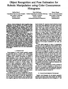
The MOPED framework: Object Recognition and Pose Estimation for Manipulation Alvaro Collet

∗

Manuel Martinez

†

Siddhartha S. Srinivasa

‡

Abstract We present MOPED, a framework for Multiple Object Pose Estimation and Detection that seamlessly integrates single-image and multi-image object recognition and pose estimation in one optimized, robust, and scalable framework. We address two main challenges in computer vision for robotics: robust performance in complex scenes, and low latency for real-time operation. We achieve robust performance with Iterative ClusteringEstimation (ICE), a novel algorithm that iteratively combines feature clustering with robust pose estimation. Feature clustering quickly partitions the scene and produces object hypotheses. The hypotheses are used to further refine the feature clusters, and the two steps iterate until convergence. ICE is easy to parallelize, and easily integrates single- and multi-camera object recognition and pose estimation. We also introduce a novel object hypothesis scoring function based on M-estimator theory, and a novel pose clustering algorithm that robustly handles recognition outliers. We achieve scalability and low latency with an improved feature matching algorithm for large databases, a GPU/CPU hybrid architecture that exploits parallelism at all levels, and an optimized resource scheduler. We provide extensive experimental results demonstrating state-of-the-art performance in terms of recognition, scalability, and latency in real-world robotic applications.

1

Introduction

Figure 1: Recognition of real-world scenes. (Top) Highcomplexity scene. MOPED finds 27 objects, including partiallyThe task of estimating the pose of a rigid object model from a occluded, repeated and non-planar objects. Using a database single image is a well studied problem in the literature. In the of 91 models and an image resolution of 1600 × 1200, MOPED case of point-based features, this is known as the Perspectiveprocesses this image in 2.1 seconds. (Bottom) Medium comn-Point (PnP) problem (Fischler and Bolles, 1981), for which plexity scene. MOPED processes this 640 × 360 image in 87 ms many solutions are available, both closed-form (Lepetit et al., and finds all known objects (The undetected green soup can is 2008) and iterative (Dementhon and Davis, 1995). Assuming not in the database). that enough perfect correspondences between 2D image features and 3D model features are known, one only needs to use the PnP solver of choice to obtain an estimation of an object’s pose. When noisy measurements are considered, non∗ A. Collet is with The Robotics Institute, Carnegie Mellon University, linear least-squares minimization techniques (e.g. Levenberg5000 Forbes Ave., Pittsburgh, PA - 15213, USA. {acollet}@cs.cmu.edu Marquardt (Marquardt, 1963)) often provide better pose esti† M. Martinez is with The Robotics Institute, Carnegie Mellon University, 5000 Forbes Ave., Pittsburgh, PA - 15213, USA. mates. Given that such techniques require good initialization, a {manelm}@cs.cmu.edu closed-form PnP solver is often used to initialize the non-linear ‡ Siddhartha S. Srinivasa Intel Labs Pittsburgh 4720 minimizer. Forbes

Avenue,

Suite

410,

Pittsburgh,

PA

-

15213,

USA.

The very related task of recognizing a single object and de-

{siddhartha.srinivasa}@intel.com

1

The International Journal of Robotics Research, April, 2011

termining its pose from a single image requires solving two sub-problems: finding enough correct correspondences between image features and model features, and estimating the model pose that best agrees with that set of correspondences. Even with highly discriminative locally invariant features, such as SIFT (Lowe, 2004) or SURF (Bay et al., 2008), mismatched correspondences are inevitable, forcing us to utilize robust estimation techniques such as M-estimators or RANSAC (Fischler and Bolles, 1981) in most modern object recognition systems. A comprehensive overview of model-based 3D object recognition/tracking techniques is available at Lepetit and Fua (2005). The problem of model-based 3D object recognition is mature, with a vast literature behind, but it is far from solved in its most general form. Two problems greatly influence the performance of any recognition algorithm. The first problem is scene complexity. This can arise due to feature count, with both extremes (too many features, or too few) significantly decreasing recognition rate. Related is the issue of repeated objects: the matching ambiguity introduced by repeated instances of an object presents an enormous challenge for robust estimators, as the matched features might belong to different object instances despite being correct. Solutions such as grouping (Lowe, 1987), interpretation trees (Grimson, 1991) or image space clustering (Collet et al., 2009) are often used, but false positives often arise from algorithms not being able to handle unexpected scene complexity. Fig. 1 shows an example of an image of high complexity and multiple repeated objects correctly processed by MOPED. The second problem is that of scalability and system latency. In systems that operate online, a trade-off between recognition performance and latency must be reached, depending on the requirements for each specific task. In robotics, the reaction time of robots operating in dynamic environments is often limited by the latency of their perception (e.g. (Srinivasa et al., 2010, WillowGarage, 2008)). Increasing the volume of input data to process (e.g. increasing the image resolution, using multiple cameras) usually results in a severe penalty in terms of processing time. Yet, with cameras getting better, cheaper, and smaller, multiple high resolution views of a scene are often easily available. For example, our robot HERB has, at various times, been outfitted with cameras on its shoulder, in the palm, on its ankle-high laser, as well as with a stereo pair. Multiple views of a scene are often desirable, because they provide depth estimation, robustness against line-of-sight occlusions, and an increased effective field of view. Fig. 2 shows MOPED applied on a set of three images for grasping. Also, the higher resolution can potentially improve the recognition of complicated objects and the accuracy of pose estimation algorithms, but often at a steep penalty cost, as the extra resolution often causes an increase in the number of false positives as well as severe degradation in terms of latency and throughput. In this paper, we address these two problems in model-based 3D object recognition through multiple novel contributions, both algorithmic and architectural. We provide a scalable framework for object recognition specifically designed to address increased scene complexity, limit false positives, and uti-

Figure 2: Object grasping in a cluttered scene using MOPED. (Top) Scene observed by a set of three cameras. (Bottom) Our robotic platform HERB (Srinivasa et al., 2010) in the process of grasping an object, using only the pose information from MOPED. lize all computing resources to provide low latency processing for one or multiple simultaneous high-resolution images. The Iterative Clustering-Estimation (ICE) algorithm is our most important contribution to handle scenes with high complexity and keep latency low. In essence, ICE jointly solves the correspondence and pose estimation problems through an iterative procedure. ICE estimates groups of features that are likely to belong to the same object through clustering, and then searches for object hypotheses within each of the groups. Each hypothesis found is used to refine the feature groups that are likely to belong to the same object, which in turn helps finding more accurate hypotheses. The iteration of this procedure focuses the object search only in the regions with potential objects, avoiding the waste of processing power in unlikely regions. In addition, ICE allows for an easy parallelization and the integration of multiple cameras in the same joint optimization. Another important contribution of this paper is a robust metric to rank object hypotheses based on M-estimator theory. A common metric used in model-based 3D object recognition is the sum of reprojection errors. However, this metric prioritizes objects that have been detected with the least amount of information, since each additional recognized object feature is bound to increase the overall error. Instead, we propose a quality metric that encourages objects to have as most correspondences as possible, thus achieving more stable estimated poses. This metric is relied upon in the clustering iterations within ICE, and is specially useful when coupled with our novel pose clustering algorithm. The key insight behind our pose clustering algorithm 2


(M = 1) and a camera-centric world (T1 = I4 , where I4 is a 4 × 4 identity matrix).

—called Projection Clustering— is that our object hypotheses have been detected from camera data, which might be noisy, ambiguous and/or contain matching outliers. Therefore, instead of using a regular clustering technique in pose space (using e.g. Mean Shift (Cheng, 1995) or Hough Transforms (Olson, 1997)), we evaluate each type of outlier and propose a solution that handles incorrect object hypotheses and effectively merges their information with those that are most likely to be correct. This work also tackles the issues of scalability, throughput and latency, which are vital for real-time robotics applications. ICE enables easy parallelism in the object recognition process. We also introduce an improved feature matching algorithm for large databases that balances matching accuracy and logarithmic complexity. Our GPU/CPU hybrid architecture exploits parallelism at all levels. MOPED is optimized for bandwidth and cache management and SIMD instructions. Components like feature extraction and matching have been implemented on a GPU. Furthermore, a novel scheduling scheme enables the efficient use of symmetric multiprocessing(SMP) architectures, utilizing all available cores on modern multi-core CPUs. Our contributions are validated through extensive experimental results demonstrating state-of-the-art performance in terms of recognition, pose estimation accuracy, scalability, throughput and latency. Five benchmarks and a total of over 6000 images are used to stress-test every component of MOPED. The different benchmarks are executed in a database of 91 objects, and contain images with up to 400 simultaneous objects, high-definition video footage, and a multi-camera setup. Preliminary versions of this work have been published at Collet et al. (2009), Collet and Srinivasa (2010), Martinez et al. (2010). Additional information, videos, and the full source code of MOPED are available online at http://personalrobotics. intel-research.net/projects/moped.

2

2.2

Input: object models

Each object to be recognized by MOPED first goes through an offline learning stage, in which a sparse 3D model of the object is created. First, a set of images is taken with the object in various poses. Reliable local descriptors are extracted from natural features using SIFT(Lowe, 2004), which have proven to be one of the most distinctive and robust local descriptors across a wide range of transformations (Mikolajczyk and Schmid, 2005). Alternative descriptors (e.g. SURF(Bay et al., 2008), ferns(Ozuysal et al., 2010)) can also be used. Using structure from motion (Szeliski and Kang, 1994) on the matched SIFT keypoints, we merge the information from each training image into a sparse 3D model. Each 3D point is linked to a descriptor that is produced from clustering individual matched descriptors in different views. Finally, proper alignment and scale for each model are computed to match the real object dimensions and define an appropriate coordinate frame, which for simplicity is defined at the object’s center. Let O be a set of object models. Each object model is defined by its object identity o and a set of features Fo O = {o, Fo } Each feature is [X, Y, Z]T in the scriptor D, whose scriptor used, e.g. SURF. That is,

Fo = {F1;o , . . . , Fi;o , . . . , FN ;o }.

(2)

represented by a 3D point location P = object’s coordinate frame and a feature dedimensionality depends on the type of dek = 128 if using SIFT or k = 64 if using

Fi;o = {Pi;o , Di;o }

Pi;o ∈ R3 , Di;o ∈ Rk .

(3)

The S union of all features from all objects in O is defined as F = o∈O Fo .

Problem formulation

The goal of MOPED is the recognition of objects from images 2.3 Output: recognized objects given a database of object models, and the estimation of the pose of each recognized object. In this section, we formalize The output of MOPED is a set of object hypotheses H. Each these inputs and outputs and introduce the terminology we use object hypothesis Hh = {o, Th } is represented by an object identity o and a 4 × 4 matrix Th that corresponds to the pose throughout the paper. of the object with respect to the world reference frame.

2.1

Input: images

3

The input to MOPED is a set I of M images

Iterative Clustering-Estimation

(1) The task of recognizing objects from local features in images requires solving two sub-problems: the correspondence problem In the general case, each image is captured with a different and the pose estimation problem. The correspondence problem calibrated camera. Therefore, each image Im is defined by a refers to the accurate matching of image features to features 3 × 3 matrix of intrinsic camera parameters Km , a 4 × 4 matrix that belong to a particular object. The pose estimation problem of extrinsic camera parameters Tm with respect to a known refers to the generation of object poses that are geometrically consistent with the found correspondences. world reference frame, and a matrix of pixel values gm . MOPED is agnostic to the number of images M . In other The inevitable presence of mismatched correspondences words, it is equally valid in both an extrinsically calibrated forces us to utilize robust estimation techniques, such as Mmulti-camera setup, and in the simplified case of a single image estimators or RANSAC (Fischler and Bolles, 1981). In the I = {I1 , . . . , Im , . . . , IM }

Im = {Km , Tm , gm }.

3


Figure 3: Illustration of two ICE iterations. Colored outlines represent estimated poses. (a) Feature extraction and matching. (b) Feature clustering. (c) Hypothesis generation. (d-e) Cluster clustering. (f) Pose refinement. (g) Final result. presence of repeated objects in a scene, the correspondence problem cannot be solved in isolation, as even perfect image-tomodel correspondences need to be linked to a particular object instance. Robust estimation techniques often fail as well in the presence of this increased complexity. Solutions such as grouping (Lowe, 1987), interpretation trees (Grimson, 1991) or image space clustering (Collet et al., 2009) alleviate the problem of repeated objects by reducing the search space for object hypotheses.

The Estimation step computes object hypotheses given clusters of features (as shown in Fig. 3.c and Fig. 3.f). Each cluster can potentially generate one or multiple object hypotheses, and also contain outliers that cannot be used for any hypothesis. A common approach for hypothesis generation is the use of RANSAC along with a pose estimation algorithm, although other approaches are equally valid. In RANSAC, we choose subsets of features at random within the cluster, then hypothesize an object pose that best fits the subset of features, and finally The Iterative Clustering-Estimation (ICE) algorithm at the check how many features in the cluster are consistent with the heart of MOPED aims to jointly solve the correspondence and pose hypothesis. This process is repeated multiple times and a pose estimation problems in a principled way. Given initial set of object hypotheses is generated for each cluster. The adimage-to-model correspondences, ICE iteratively executes clus- vantage of restricting the search space to that of feature clusters tering and pose estimation to progressively refine which features is the higher likelihood that features from only one object inbelong to each object instance, and to compute the object poses stance are present, or at most a very limited number of them. that best fit each object instance. The algorithm is illustrated This process can be performed regardless of whether the features belong to one or multiple images. in Fig. 3. Given a scene with a set of matched features, (Fig. 3.a), the Clustering step generates groups of image features that are likely to belong to a single object instance (Fig. 3.b). If prior object pose hypotheses are available, features consistent with each object hypothesis are used to initialize distinct clusters. Numerous object hypotheses are generated for each cluster (Fig. 3.c). Then, object hypotheses are merged together if their poses are similar (Fig. 3.d), thus uniting their feature clusters into larger clusters that potentially contain all information about a single object instance (Fig. 3.e). With multiple images, the use of a common reference frame allows us to link object hypotheses recognized in different images, and thus create multi-image feature clusters. If prior object pose hypotheses are not available (i.e. at the first iteration of ICE), we use the density of local features matched to an object model as a prior, with the intuition that groups of features spatially close together are more likely to belong to the same object instance than features spread across all images. Thus, we initialize ICE with clusters of features in image space (x, y), as seen in Fig. 3.b.

The set of hypotheses from the Estimation step are then utilized to further refine the membership of each feature to each cluster (Fig. 3.d-e). The whole process is iterated until convergence, which is reached when no features change their membership in a Clustering step (Fig. 3.f).

In practice, ICE requires very few iterations until convergence, usually as little as 2 for setups with one or a few simultaneous images. Parallelization is easy, since the initial steps are independent for each cluster in each image and object type. Therefore, large sets of images can be potentially integrated into ICE with very little impact on overall system latency. Two ICE iterations are required for increased robustness and speed in setups ranging from one to a few simultaneous images, while further iterations of ICE might potentially be necessary if tens or hundreds of simultaneous images are to be processed. 4


3.1

ICE as Expectation-Maximization

be considered if working with a larger set of simultaneous images. It is interesting to note the conceptual similarity between ICE 1. Feature Extraction. Salient features are extracted from and the well-known Expectation-Maximization (EM) (Demp- each image. We represent images I as sets of local features f . m ster et al., 1977) algorithm, particularly in the learning of Gaus- Each image I ∈ I is processed independently, so that m sian Mixture Models (GMM) (Redner and Walker, 1984). EM is an iterative method for finding parameter estimates in staIm = {Km , Tm , fm } fm = FeatExtract(gm ). (4) tistical models than contain unobserved latent variables, alterEach individual local feature fj;m from image m is defined nating between expectation (E) and maximization (M) steps. T The expectation (E) step computes the expected value of the by a 2D point location pj;m = [x, y] and its corresponding log-likelihood using the current estimate for the latent vari- feature descriptor dj;m ; that is, ables. The maximization (M) step computes the parameters fm = {f1;m , . . . , fj;m , . . . , fJ;m } fj;m = {pj;m , dj;m }. (5) that maximize the expected log-likelihood found on the E step. These parameter values determine the latent variable distribuWe define the S union of all extracted local features from all tion in the next E step. In Gaussian Mixture Models, the EM M images m as f = m=1 fm . algorithm is applied to find a set of Gaussian distributions that 2. Feature Matching. One-to-one correspondences are best fits a set of data points. The E step computes the expected created between extracted features in the image set and object membership of each data point to one of the Gaussian distrifeatures stored in the database. For efficiency, approximate butions, while the M step computes the parameters for each matching techniques can be used, at the cost of a decreased distribution given the memberships computed in the E step. recognition rate. Let C be a correspondence between an image Then, the E step is repeated with the updated parameters to feature fj;m and a model feature Fi;o , such that recompute new membership values. The entire procedure is ( repeated until model parameters converge. (fj;m , Fi;o ) , if fj;m ↔ Fi;o o Cj,m = . (6) Despite the mathematical differences, the concept behind ∅, otherwise ICE is essentially the same. The problem of object recognition in the presence of severe clutter and/or repeated objects The set of correspondences for a given object o and image m S o can be interpreted as one of estimation of model parameters is represented as Com = ∀j Cj;m . The sets Sof correspondences o o —the pose of a set of objects—, where the model depends on Cm , C are defined equivalently as Cm = ∀j,o Cj;m and Co = S o unobserved latent variables —the correspondences of image fea∀j,m Cj;m . tures to particular object instances—. Under this perspective, 3. Feature Clustering. Features matched to a particular the Clustering step of ICE computes the expected membership object are clustered in image space (x, y), independently for of each local feature to one of the object instances, while the each image. Given that spatially close features are more likely Estimation step computes the best object poses given the fea- to belong to the same object instance, we cluster the set of ture memberships computed in the Clustering step. Then, the feature locations p ∈ Com , producing a set of clusters that group entire procedure is repeated until convergence. If our object features spatially close together. models were Gaussian distributions, ICE and GMMs would be Each cluster Kk is defined by an object identity o, an image virtually equivalent. index m, and a subset of the correspondences to object O in image Im , that is,

4

Kk = {o, m, Ck ⊂ Com }.

The MOPED Framework

(7)

The set of all clusters is expressed as K. 4. Estimation #1: Hypothesis Generation. Each cluster is processed in each image independently in search of objects. RANSAC and Levenberg-Marquardt (LM) are used to find object instances that are loosely consistent with each object’s geometry in spite of outliers. The number of RANSAC iterations is high and the number of LM iterations is kept low, so that we discover multiple object hypotheses with coarse pose estimation. At this step, each hypothesis h consists of

This section contains a brief summary of the MOPED framework and its components. Each individual component is explored in depth in subsequent sections. The steps itemized below compose the basic MOPED framework for the typical requirements of a robotics application. In essence, MOPED is comprised of a single feature extraction and matching step per image, and multiple iterations of Iterative Clustering-Estimation (ICE) that efficiently perform object recognition and pose estimation per object in a bottom-up approach. Assuming the most common setup of object recognition, utilizing a single or a small set of images (i.e. less than 10), we fix ICE to compute two full Clustering-Estimation iterations plus a final cluster merging to remove potential multiple detections that might have not yet converged. This way, we ensure a good trade-off between high recognition rate and reduced system latency, but a greater number of iterations should

h = {o, k, Th , Ch ⊂ Ck },

(8)

where o is the object identity of hypothesis h, k is a cluster index, Th is a 4×4 transformation matrix that defines the object hypothesis pose with respect to the world reference frame, and Ch is the subset of correspondences that are consistent with hypothesis h. 5


5. Cluster Clustering. As the same object might be present in multiple clusters and images, poses are projected from the image set onto a common coordinate frame, and features consistent with a pose are re-clustered. New, larger clusters are created, that often contain all consistent features for a whole object across the entire image set. These new clusters contain KK = {o, CK ⊂ Co }.

(9)

6. Estimation #2: Pose Refinement. After Steps 4 and 5, most outliers have been removed, and each of the new clusters is very likely to contain features corresponding to only one instance of an object, spanned across multiple images. The RANSAC procedure is repeated for a low number of iterations, and poses are estimated using LM with a larger number of iterations to obtain the final poses from each cluster that are consistent with the multi-view geometry. Each multi-view hypothesis H is defined by H = {o, TH , CH ⊂ CK },

Figure 4: Example of highly cluttered scene and the importance of clustering. (Top-left) Scene with 9 overlapping notebooks. (Bottom-left) Recovered poses for notebooks with MOPED. (Right) Clusters of features in image space. outliers. However, both of them fail in the presence of heavy clutter and multiple objects, in which only a small percentage of the matched correspondences belong to the same object instance. To overcome this limitation, we propose the creation of object priors based on the density of correspondences across the image, by exploiting the assumption that areas with a higher concentration of correspondences for a given model are more likely to contain an object than areas with very few features. Therefore, we aim to create subsets of correspondences within each image that are reasonably close together and assume they are likely to belong to the same object instance, avoiding the waste of computation time in trying to relate features spread all across the image. We can accomplish this goal by seeking the modes of the density distribution of features in image space. A well-known technique for this task is Mean Shift clustering (Cheng, 1995), which is a particularly good choice for MOPED because no fixed number of clusters needs to be specified. Instead, a radius parameter needs to be chosen, that intuitively selects how close two features must in order to be part of the same cluster. Thus, for each object in each image independently, we cluster the set of feature locations p ∈ Com (i.e. pixel positions p = (x, y)), producing a set of clusters K that contain groups of features spatially close together. Clusters that contain very few features, those in which no object can be recognized, are discarded, thus considering the features as outliers and discarding them as well. The advantage of using Mean Shift clusters as object priors is illustrated in Fig. 4. In Fig. 4.(top-left) we see an image with 9 notebooks. As a simple example, let us imagine that all notebooks have the same number of correspondences, and that 70% of those correspondences are correct, i.e., that the global inlier # inliers ratio w = # points = 0.7. The inlier ratio for a particular notebook is then wobj = # wobj = 0.0778. The number of iterations k theoretically required (Fischler and Bolles, 1981) to find one particular instance of a notebook with probability p is

(10)

where o is the object identity of hypothesis H, TH is a 4 × 4 transformation matrix that defines the object hypothesis pose with respect to the world reference frame, and CH is the subset of correspondences that are consistent with hypothesis H. 7. Pose Recombination. A final merging step removes any multiple detections that might have survived, by merging together object instances that have similar poses. A set of hypotheses H, with Hh = {o, TH }, is the final output of MOPED.

5

Addressing Complexity

In this section, we provide an in-depth explanation of our contributions to address complexity that have been integrated in the MOPED object recognition framework, and how each of our contributions relate to the Iterative Clustering-Estimation procedure.

5.1

Image Space Clustering

The goal of Image Space Clustering in the context of object recognition is the creation of object priors based solely on image features. In a generic unstructured scene, it is infeasible to attempt the recognition of objects with no higher-level reasono ing than the image-model correspondences Cj,m = (fj;m , Fi;o ). Correspondences for a single object type o may belong to different object instances, or may be matching outliers. Multicamera setups are even more uncertain, since the amount of image features increases dramatically, and so does the probability of finding multiple repeated objects in the combined set of images. Under these circumstances, the ability to compute a prior over the image features is of utmost importance, in order to evaluate which of the features are likely to belong to the same object instance, and which of them are likely to be outliers. RANSAC (Fischler and Bolles, 1981) and M-estimators are often the methods of choice to find models in the presence of

k=

6

log(1 − p) , log(1 − (wobj )n )

(11)


• The minimum distance error in each of the correspondences.

where n is the number of inliers for a successful detection. If we require n = 5 inliers and a probability p = 0.95 of finding a particular notebook, then we should perform k = 1.05M iterations of RANSAC. On the other hand, clustering the correspondences in smaller sets as in Fig. 4.(right) means that fewer notebooks (at most 3) are present in a given cluster. In such a scenario, finding one particular instance of a notebook with 95% probability requires 16, 586 and 4386 iterations when 1, 2 and 3 notebooks, resp., are present in a cluster, at least three orders of magnitude lower than the previous case.

5.2

The sum of reprojection errors in Eq. (19) is not a good evaluation metric according to these requirements, as this error is bound to increase whenever an extra correspondence is added. Therefore, the sum of reprojection errors favors hypotheses with the least amount of correspondences, which can lead to choosing spurious hypotheses over more desirable ones. In contrast, we define a robust estimator based on the Cauchy distribution that balances the two criteria stated above. Consider the set of consistent correspondences Ch for a given object hypothesis, where each correspondence Cj = (fj;m , Fi;o ). Assume the corresponding features in Cj have locations in an image pj and in an object model Pj . Let dj = d(pj , Th Pj ) be an error metric that measures the distance between a 2D point in an image and a 3D point from hypothesis h with pose Th (e.g. reprojection, backprojection errors). Then, the Cauchy distribution ψ(dj ) is defined by

Estimation #1: Hypothesis generation

In the first Estimation step of ICE, our goal is to generate coarse object hypotheses from clusters of features, so that the object poses can be used to refine the cluster associations. In general, each cluster Kk = {o, m, Ck ⊂ Com } may contain features from multiple object hypotheses as well as matching outliers. In order to handle the inevitable presence of matching outliers, we use the robust estimation procedure RANSAC. For a given cluster Kk , we choose a subset of correspondences C ⊂ Ck and estimate an object hypothesis with the best pose that minimizes the sum of reprojection errors (see Eq. (18)). We minimize the sum of reprojection errors via a standard LevenbergMarquardt (LM) non-linear least squares minimization. If the amount of correspondences in Ck consistent with the hypothesis is higher than a threshold , we create a new object instance and refine the estimated pose using all consistent correspondences in the optimization. We then repeat this procedure until the amount of unallocated points is lower than a threshold, or the maximum number of iterations has been exceeded. By repeating this procedure for all clusters in all images and objects, we produce a set of hypotheses h, where each hypothesis h = {o, k, Th , Ch ⊂ Ck }. At this stage, we wish to obtain a set of coarse pose hypotheses to work with, as fast as possible. We require a large number of RANSAC iterations to detect as many object hypotheses as possible, but we can use a low maximum number of LM iterations and loose threshold when minimizing the sum of reprojection errors. Accurate pose will be achieved in later stages of MOPED. The initialization of LM for pose estimation can be implemented with either fast PnP solvers such as the ones proposed in (Collet et al., 2009, Lepetit et al., 2008) or even completely at random within the space of possible poses (e.g. some distance in front of the camera). Random initialization is the default choice for MOPED, as it is more robust to the pose ambiguities that sometimes confuse PnP solvers.

ψ(dj ) = 1+

1 2 ,

(12)

dj σ

where σ 2 parameterizes the cut-off distance at which ψ(dj ) = 0.5. In our case, the distance metric dj is the reprojection error measured in pixels. This distribution is maximal when dj = 0, i.e. ψ(0) = 1, and monotonically decreases to zero when a pair of correspondences are infinitely away from each other, i.e. ψ(∞) = 0. The Quality Score Q for a given object hypothesis h is then defined as a summation over the Cauchy scores ψ(dj ) for all correspondences:

Q(h) =

X ∀j:Cj ∈Ch

ψ(dj ) =

1

X ∀Cj ∈Ch

1+

d2 (pj ,Th Pj ) σ2

.

(13)

The Q-Score has a lower bound at 0, if a given hypothesis has no correspondences or if all its correspondences have infinite error, and has an upper bound at |O|, which is the total number of correspondences for model O. This score allows us to reliably rank our object hypotheses and evaluate their strength. The cut-off distance σ may be either a fixed value, or adjusted at each iteration via robust estimation techniques (Zhang, 1997), depending on the application. Robust estimation techniques require a certain minimum outlier/inlier ratio to work properly ( ##outliers inliers < 1 in all cases), known as the breaking point of a robust estimator (Huber, 1981). In the case of MOPED, the outlier/inlier ratio is often well over the breaking point of 5.3 Hypothesis Quality Score any robust estimator, especially when multiple instances of an It is useful at this point to introduce a robust metric to quan- object are present; as a consequence, robust estimators might titatively compare the goodness of multiple object hypotheses. result in unrealistically large values of σ in complex scenes. The desired object hypothesis metric should favor hypotheses Therefore, we choose to set a fixed value for the cut-off parameter, σ = 2 pixels, for a good balance between encouraging a with: large number of correspondences while keeping their reprojection error low. • The most amount of consistent correspondences. 7


5.4

Cluster Clustering

outliers in the feature matching process. To the contrary, most outlier detections are artifacts of the projection of a 3D scene The disadvantage of separating the image search space into a into a 2D image when captured by a perspective camera. In set of clusters is that the produced pose hypotheses may be particular, we can distinguish two different cases: generated with only partial information from the scene, given that information from other clusters and other views is not • A group of correct matches whose 3D configuration is deconsidered in the initial Estimation step of ICE. However, once generate or near-degenerate (e.g. a group of 3D points that a rough estimate of the object poses is known, we can merge are almost collinear), incorrectly grouped with one single the information from multiple clusters and multiple views to matching outlier. In this case, the output pose is largely obtain sets of correspondences that contain all features from a determined by the location of the matching outlier, which single object instance (see Fig. 3). causes arbitrarily erroneous hypotheses to be accepted as Multiple alternatives are available to group similar hypothecorrect. ses into clusters. In this section, we propose a novel hypothesis clustering algorithm called Projection Clustering, in which we • Pose ambiguities in objects with planar surfaces. The perform correspondence-level grouping from a set of object hysum of reprojection errors in planar surfaces may contain potheses h and provide a mechanism to robustly filter any pose two complementary local minima in some configurations outliers. of pose space(Schweighofer and Pinz, 2006), which often For comparison, we introduce a simpler Cluster Clustering causes the appearance of two distinct and partially overscheme based on Mean Shift, and analyze the computational lapping object hypotheses. These hypotheses are usually complexity of both schemes to conclude in which cases we might too distant in pose space to be grouped together. prefer one over the other. 5.4.1

The false positives output in the pose hypothesis generation are often too distant from any correct hypothesis in the scene, and cannot be merged using regular clustering techniques (e.g. Mean Shift). However, the point features that generated those false positives are usually correct, and they can provide valuable information to some of the correct object hypotheses. In Projection clustering, we process each point feature individually, and assign them to the strongest pose hypothesis to which they might belong. Usually, spurious poses only contain a limited number of consistent point features, thus resulting in lower Qscores (Section 5.3) than correct object hypotheses. By transferring most of the point features to the strongest object hypotheses, we not only utilize the extra information available in the scene for increased accuracy, but also filter most false positives by lowering their number of consistent points below the required minimum. The first step in Projection clustering is the computation of Q-Scores for all object hypotheses h. We generate a pool of potential correspondences Co that contains all correspondences for a given object type that are consistent with at least one pose hypothesis. Correspondences from all images are included in Co . We compute the Quality score for each hypothesis h from all correspondences Cj = (fj , Fj ) such that Cj ∈ Co .

Mean Shift clustering on pose space

A straightforward hypothesis clustering scheme is to perform Mean Shift clustering on all hypotheses h = {o, k, Th , Ch ⊂ Ck } for a given object type o. In particular, we cluster the pose hypotheses Th in pose space. In order to properly measure distances between poses, it is convenient to parameterize rotations in terms of quaternions and project them in the same half of the quaternion hypersphere prior to clustering, using then Mean Shift on the resulting 7-dimensional poses. After this procedure, we merge the correspondence clusters Ch of those poses that belong to the same pose cluster TK . [ CK = Ch (14) Th ∈TK

This produces clusters KK = {o, CK ⊂ Co } whose correspondence clusters span over multiple images. In addition, the centroid of each pose cluster TK can be used as initialization for the following Estimation iteration of ICE. At this point, we can discard all correspondences not consistent with any pose hypothesis, thus filtering many outliers and reducing the search space for future iterations of ICE. The computational complexity of Mean Shift is O(dN 2 t), where d = 7 is the dimensionality of the clustered data, N = |h| is the total number of hypotheses to cluster, and t is the number of iterations that Mean Shift requires. In practice, the number of hypotheses is often fairly small, and t ≤ 100 in our implementation. 5.4.2

Q(h) =

X ∀j:Cj ∈Co

ψ(dj ) =

1

X ∀Cj ∈Co

1+

d2 (pj ,Th Pj ) σ2

(15)

For each potential correspondence Cj in Co , we define a set of likely hypotheses hj as the set of those hypotheses h whose reprojection error is lower than a threshold γ. This threshold can be interpreted as an attraction coefficient; large values of γ lead to heavy transference of correspondence to strong hypotheses, while small values cause few correspondences to transfer from one hypothesis to another. In our experiments, a large threshold γ of 64 pixels is used.

Projection clustering

Mean Shift provides basic clustering in pose space, and works well when multiple correct detections of an object are present. However, it is possible that spurious false positives are detected in the hypothesis generation step. It is important to realize that these false positives are very rarely exclusively due to random 8


Table 1: Mean Recognition per Image: Mean Shift vs Projection Clustering, in the Simple Movie Benchmark (see SecAt this point, the relation between correspondences Cj and tion 6.2.3 for details). hypotheses h is broken. In other words, we empty the set of correspondences Ch for each hypothesis h, so that Ch = ∅. Then, we re-assign each correspondence Cj ∈ Co to the pose True Pos. False Pos. False Neg. hypothesis h within hj with stronger overall Q-Score: Mean Shift 10.92 3.32 1.97 P.Clust. (Q-Score) 11.3 2.29 1.59 Ch ← Cj : h = arg max Q(h) (17) P.Clust. (Reproj) 11.05 7.4 1.84 h∈hj P.Clust. (Avg Reproj) 10.88 7.81 2.01 Finally, it is important to check the remaining number of corP.Clust. (# Corresp) 3.6 9.82 9.29 respondences that each object hypothesis has after Projection h ∈ hj ⇐⇒ d2 (pj , Th Pj ) < γ

(16)

clustering. Pose hypotheses that retain less than a minimum number of consistent correspondences are considered outliers and therefore discarded. The Projection Clustering algorithm we propose has a computational complexity O(M N I), where M = |C| is the total number of correspondences to process, N = |h| is the number of pose hypotheses and I = |I| is the total number of images. Comparing this with the complexity O(dN 2 t) of Mean Shift, we see that the only advantage of Mean Shift in terms of computational cost would be in the case of object models with enormous numbers of features and many high resolution images, so that O(M N I) O(dN 2 t). While offering a similar computational complexity, the advantage of Projection Clustering with respect to Mean Shift is in terms of improved robustness and outlier detection, both of which are essential for handling increased complexity in MOPED.

recognizes and estimates the pose of 87.6% of the objects in the dataset. Mean Shift is the second best performer, but the increased false positive rate is mainly due to pose ambiguities that cannot be resolved and produce spurious detections. The different hypothesis ranking schemes critically impact the overall performance of Projection Clustering, as multiple poses often need to be merged after the first Clustering-Estimation iteration. Ranking spurious poses over correct poses results in an increased number of false positives, as Projection Clustering is unable to merge object hypothesis properly. While Q-Score is able to estimate the best pose out a set of multiple detections, Reprojection and Avg. Reprojection select sub-optimal poses that contain just a few points, often including outliers. This behavior severely impacts the performance of Projection Clustering, which barely merges any pose hypotheses and produces 5.4.3 Performance Comparison an increased number of false positives. The Num. Correspondences metric prefers hypotheses with many consistent matches In this experiment, we compare the recognition performance of in the scene, and Projection Clustering merges hypotheses corMOPED when using the two Cluster Clustering approaches exrectly. Unfortunately, the chosen best hypotheses are in most plained in this section. In addition, and given that Projection cases incorrect due to ambiguities, estimating only 28% of the Clustering depends on the behavior of a hypothesis ranking poses correctly. It must be noted that in simple scenes with a mechanism, we implement four different ranking mechanisms few unoccluded objects all the evaluated metrics perform simand compare their performance. The first ranking mechanism ilarly well. Projection Clustering and Q-Score, however, showis our own Q-Score introduced in Section 5.3, while the other case increased robustness when working with the most complex approaches considered are the sum of reprojection errors, the scenes. average reprojection error, and the number of consistent correspondences. The performance of MOPED when using the different Cluster Clustering and hypothesis ranking algorithms 5.5 Estimation #2: Pose Refinement is shown in Table 1, on a subset of 100 images from the Simple Movie Benchmark (Section 6.2.3) that contain a total of 1289 At the second iteration of ICE, we use the information from initial object hypotheses to obtain clusters that are most likely object instances. An object hypothesis is considered a true positive if its pose to belong to a single object instance, with very few outliers. estimate is within 5 cm and 10 degrees of the ground truth pose. For this reason, the Estimation step at the second iteration of Object hypotheses whose pose is outside this error range are ICE requires only a low number of RANSAC iterations to find considered false positives. Ground truth objects without an as- object hypotheses. In addition, we use a high number of LM sociated true positive are considered false negatives. According iterations to estimate object poses accurately. This procedure is equivalent to that of the first Estimation to these performance metrics, the appearance of pose ambiguities and misdetections is particularly critical, since they often step, being the objective function to minimize the only differproduce both a false positive –the rotational error is greater ence between the two. For a given multi-view feature clusthan the threshold– and a false negative –no pose agrees with ter KK , we perform RANSAC on subsets of correspondences C ⊂ CK and obtain pose hypotheses H = {o, TH , CH ⊂ CK } the ground truth–. The overall best-performer is Projection Clustering when us- with consistent correspondences CH ⊂ CK . The objective ing Q-Score as its hypothesis ranking metric, which correctly function to minimize can be either the sum of reprojection er9


rors (Eq. (19)) or the sum of backprojection errors (Eq. (24)). See Appendix A for a discussion on these two objective functions. We initialize the non-linear minimization of the chosen objective function using the highest-ranked pose in CK according to their Q-Scores. This non-linear minimization is performed, again, with a standard Levenberg-Marquardt non-linear least squares minimization algorithm.

5.6

6.2

Benchmarks

We present four benchmarks (Fig. 5) designed to stress test every component of our system. All benchmarks, both synthetic and real-world, provide exclusively a set of images and ground truth object poses (i.e., no synthetically computed feature locations or correspondences). We performed all experiments on a 2.33GHz quad-core Intel(R) Xeon(R) E5345 CPU, 4 GB of RAM and a nVidia GeForce GTX 260 GPU running Ubuntu 8.04 (32 bits).

Truncating ICE: Pose Recombination

An optional final step should be applied in case ICE has not converged after two iterations, in order to remove multiple detections of objects. In this case, we perform a full Clustering step as in Section 5.4, and if any hypothesis H ∈ H is updated with transferred correspondences, we perform a final LM optimization that minimizes Eq. (24) on all correspondences CH .

6.2.1

The Rotation Benchmark

The Rotation Benchmark is a set of synthetic images that contains highly cluttered scenes with up to 400 cards in different sizes and orientations. This benchmark is designed to test MOPED’s scalability with respect to the database size, while keeping a constant number of features and objects. We have generated a total of 100 independent images for different res(1400 × 1050, 1000 × 750, 700 × 525, 500 × 375 and 6 Addressing Scalability and Latency olutions 350 × 262). Each image contains from 5 to 80 different objects In this section, we present multiple contributions to optimize and up to 400 simultaneous object instances. MOPED in terms of scalability and latency. We first introduce a set of four Benchmarks designed to stress test every compo- 6.2.2 The Zoom Benchmark nent of MOPED. Each of our contributions is evaluated and The Zoom Benchmark is a set of synthetic images that proverified on this set of benchmarks. gressively zooms in on 160 cards until only 12 cards are visible. This benchmark is designed to check the scalability of MOPED 6.1 Baseline system with respect to the total number of detected objects in a scene. We generated a total of 145 independent images for different For comparison purposes, we provide results for a Baseline sysresolutions (1400 × 1050, 1000 × 750, 700 × 525, 500 × 375 and tem that implements the MOPED framework with none of the 350 × 262). Each image contains from 12 to 80 different objects optimizations described in Section 6. In each case, we have and up to 160 simultaneous object instances. This benchmark tried to choose the most widespread publicly available code lisimulates a board with 160 cards seen by a 60◦ FOV camera at braries for each task. In particular, the following configuration distances ranging from 280mm to 1050mm. The objects were is used as the baseline for our performance experiments: chosen to have the same number of features at each scale. Each Feature Extraction with an OpenMP-enabled, CPUimage has over 25000 features. optimized version of SIFT we have developed. Feature matching with a publicly available implementation of ANN by Arya et al. (1998) and 2-NN Per Object (described 6.2.3 The Simple Movie Benchmark in Section 6.3.1). Synthetic benchmarks are useful to test a system in controlled Image Space clustering with a publicly available C imple- conditions, but are a poor estimator of the performance of a mentation of Mean Shift (Doll´ ar and Rabaud, 2010). system in the real world. Therefore, we provide two real-world Estimation #1 with 500 iterations of RANSAC and up to scenarios for algorithm comparison. The Simple Movie Bench100 iterations of the Levenberg-Marquardt (LM) implementa- mark consists of a 1900-frame movie at 1280 x 720 resolution, tion from Lourakis (2010), optimizing the sum of reprojection each image containing up to 18 simultaneous object instances. errors in Eq. (18). Cluster Clustering with Mean Shift, as described in Sec6.2.4 The Complex Movie Benchmark tion 5.4.1. Estimation #2 with 24 iterations of RANSAC and up to The Complex Movie Benchmark consists of a 3542-frame movie 500 iterations of LM, optimizing the sum of backprojection at 1600 x 1200 resolution, each image containing up to 60 sierrors in Eq. (24). The particular number of iterations of multaneous object instances. The database contains 91 models RANSAC in this step is not a critical factor, as most objects and 47342 SIFT features when running this benchmark. It are successfully recognized in the first 10-15 iterations. It is is noteworthy that the scenes in this video present particuuseful, however, to use a multiple of the number of concurrent larly complex situations, including: several objects of the same threads (see Section 6.4.3) for performance reasons. model contiguous to each other, which stresses the clusterPose Recombination with Mean Shift and up to 500 iter- ing step; overlapping partially-occluded objects, which stresses ations of LM. RANSAC; and objects in particularly ambiguous poses, which 10


Figure 5: MOPED Benchmarks. For the sake of clarity, only half of the detected objects are marked. (a) The Rotation Benchmark: MOPED processes this scene 36.4x faster than the Baseline. (b) The Zoom Benchmark: MOPED processes this scene 23.4x faster than the Baseline. (c) The Simple Movie Benchmark. (d) The Complex Movie Benchmark. stresses both LM and the merging algorithm, that encounter difficulties determining which pose is preferable.

6.3

Feature Matching

Once a set of features have been extracted from input image(s), we must find correspondences between the image features and our object database. Matching is done as a nearest neighbor search in the 128-dimensional space of SIFT features. An average database of 100 objects can contain over 60,000 features. Each input image, depending on the resolution and complexity of the scene, can contain over 10,000 features. The feature matching step aims to create one-to-one correspondences between model and image features. The feature matching step is, in general, the most important bottleneck for model-based object recognition to scale to large object databases. In this section, we propose and evaluate different alternatives to maximize scalability with respect to the number of objects in the database, without sacrificing accuracy. The extension of the matching search space is, in this case, the balancing factor between accuracy and speed when finding nearest

neighbors. There are no known exact algorithms for solving the matching problem that are faster than linear search. Approximate algorithms, on the other hand, can provide massive speedups at the cost of a decreased matching accuracy, and are often used wherever speed is an issue. Many approximate approaches for finding the nearest neighbors to a given feature are based on kd-trees (e.g. ANN (Arya et al., 1998), randomized kd-trees (Silpa-Anan and Hartley, 2008), FLANN (Muja and Lowe, 2009)) or hashing (e.g. LSH (Andoni and Indyk, 2006)). A ratio test between the first two nearest neighbors is often performed for outlier rejection. We analyze the different alternatives in which these techniques are often applied to feature matching, and propose an intermediate solution that achieves a good balance between recognition rate and system latency. 6.3.1

2-NN per Object

On the one end, we can compare the image features against each model independently. If using e.g. ANN, we build a kd-tree for each model in the database once (off-line), and we match each of

11


them against every new image. This process entails a complex¯ o |)), where |fm | is the number of features Table 2: Feature matching algorithms in the Simple Movie ity of O(|fm ||O| log(|F Benchmark. GPU used as performance baseline, as it computes on the image, |O| the number of models in the database, and ¯ o | the mean number of features for each model. When |O| exact nearest neighbors. |F is large, this approach is vastly inefficient as the cost of access# Corresp: After Matching After clustering Final ing each kd-tree dominates the overall search cost. The search space is in this case very limited, and there is no degradation in GPU 3893.7 853.2 562.1 performance when new models are added to the database. We OBJ MATCH 3893.6 712.0 449.2 refer to it as OBJ MATCH. 1778.4 508.8 394.7 DB MATCH MOPED-90 3624.9 713.6 428.9 6.3.2 2-NN per Database On the other end, we can compare the image features against the whole object database. This na¨ıve alternative, which we term DB MATCH, builds just one kd-tree containing the features from all models. This solution has a complexity of ¯ o |)). The search space is in this case the whole O(|fm | log(|O||F database. While this approach is orders of magnitude faster than the previous one, every new object added to the database degrades the overall recognition performance of the system due to the presence of similar features in different objects. In the limit, if an infinite number of objects were added to the database, no correspondences would ever be found, because the ratio test between the first and second nearest neighbor would be always close to 1.

Matching Time(ms)

Objects Found

253.34 498.586 129.85 140.36

8.8 8.0 7.5 8.2

GPU OBJ MATCH DB MATCH MOPED-90

MOPED 30

MOPED 90

GPU

14

Latency (relative)

12 Latency (s)

10 8 6 4

6.3.3

Brute Force on GPU

2 0 20

40

2 1.5 1 0.5

60

80

5

10

20

40

80

40

80

Models in DB (log)

1.02 1 0.98 0.96 0.94 0.92 0.9 0.88 0.86 0.84

1.02 SIFTs per Object (relative)

Objects Found (relative)

Models in DB (lin)

1 0.98 0.96 0.94 0.92 0.9 0.88 0.86

5

10

20 Models in DB (log)

6.3.4

DB_MATCH

0 0

The advent of GPUs and their many-core architecture allows the efficient implementation of an exact feature matching algorithm. The parallel nature of the brute force matching algorithm suits the GPU, and allows it to be faster than the ANN approach when |O| is not too large. Given that this algorithm scales linearly with the number of features instead of logarithmically, we can match each model independently without performance loss.

OBJ_MATCH 2.5

40

80

5

10

20 Models in DB (log)

k-NN per Database

Alternatively, one can consider the closest k nearest neighbors instead (with k > 2). k-ANN implementations using kdtrees can provide more neighbors without significantly increasing their computational cost, as they are often a byproduct of the process of obtaining the nearest neighbor. An intermediate approach to the ones presented before is the search for k multiple neighbors in the whole database. If two neighbors from the same model are found, the distance ratio is then applied to the 2 nearest neighbors from the same model. If the nearest neighbor is the only neighbor for a given model, we apply the distance ratio with the second nearest neighbor to avoid spurious correspondences. This algorithm (with k = 90) is the default choice for MOPED.

Figure 6: Scalability of feature matching algorithms with respect to the database size, in the Rotation Benchmark at 1400 × 1050 resolution.

almost logarithmically. We show MOPED-k using k = 90 and k = 30. The value of k adjusts the speed and quality behavior of MOPED between OBJ MATCH (k = ∞) and DB MATCH (k = 2). The recognition performance of MOPED-k when using the different strategies is shown in Table 2. GPU provides an upper bound for the object recognition, as it is an exact search method. OBJ MATCH comes closest in raw matching accuracy with MOPED-90 a close second. However, the number of objects detected are nearly the same. The match6.3.5 Performance comparison ing speed of MOPED-90 is, however, significantly better than Fig. 6 compares the cost of the different alternatives on the OBJ MATCH. Feature matching in MOPED-90 thus provides Rotation Benchmark. OBJ MATCH and GPU scale linearly a significant performance increase without sacrificing much acwith respect to |O|, while DB MATCH and MOPED-k scale curacy. 12


6.4

Architecture Optimizations

Latency (ms)

Latency (ms)

Table 3: SIFT vs. SURF: Mean Recognition Performance per Our algorithmic improvements were focused mainly on boosting Image in Zoom Benchmark. the scalability and robustness of the system. The architectural improvements of MOPED are obtained as a result of an impleLatency (ms) Recognized Objects mentation designed to make the best use of all the processing SIFT 223.072 13.83 resources of standard compute hardware. In particular, we use SURF 86.136 6.27 GPU-based processing, intra-core parallelization using SIMD instructions, and multi-core parallelization. We have also carefully optimized the memory subsystem, including bandwidth 350 500 700 1000 1400 transfer and cache management. 2500 300 All optimizations have been devised to reduce the latency 250 2000 between the acquisition of an image and the output of the pose 200 1500 estimates, to enable faster response times from our robotic plat150 1000 form. 100 500

6.4.1

GPU and Embarrassingly Parallel Problems

50

0

0 SIFT-CPU

State-of-the-art CPUs, such as the Intel Core i7 975 Extreme, can achieve a peak performance of 55.36 GFLOPS, according to the manufacturer (Intel Corp., 2010). State-of-the-art GPUs, such as the ATI Radeon HD 5900, can achieve a peak performance of 4640 SP GFLOPS (AMD, 2010). To use GPU resources efficiently, input data needs to be transferred to the GPU memory. Then, algorithms are executed simultaneously on all shaders, and finally recover the results from the GPU memory. As communication between shaders is expensive, the best GPU-performing algorithms are those that can be divided evenly into a large number of simple tasks. This class of easily separable problems is called Embarrassingly Parallel Problems (EPP) (Wilkinson and Allen, 2004). GPU-Based Feature Extraction. Most feature extraction algorithms consist of an initial keypoint detection step followed by a descriptor calculation for each keypoint, both of which are EPP. Keypoint detection algorithms can process each pixel from the image independently. They may need information about neighboring pixels, but they do not typically need results from them. After obtaining the list of keypoints, the respective descriptors can also be calculated independently. In MOPED, we consider two of the most popular locally invariant features: SIFT (Lowe, 2004) and SURF (Bay et al., 2008). SIFT features have proven to be among the bestperforming invariant descriptors in the literature (Mikolajczyk and Schmid, 2005), while SURF features are considered to be a fast alternative to SIFT. MOPED uses SIFT-GPU (Wu, 2007) as its main feature extraction algorithm. If compatible graphics hardware is not detected MOPED automatically reverts back to performing SIFT extraction on the CPU, which is an OpenMPenabled, CPU-optimized version of SIFT we have developed. A GPU-enabled version of SURF, GPU-SURF (Cornelis and Van Gool, 2008), is used for comparison purposes. We evaluate the latency of the three implementations in Fig. 7. The comparison is as expected: GPU versions of both SIFT and SURF provide tremendous improvements over their non-GPU counterparts. Table 3 compares the object recognition performance of SIFT and SURF: SURF proves to be 2.59x

SIFT-GPU

SIFT-GPU

SURF-GPU

Figure 7: SIFT-CPU vs. SIFT-GPU vs. SURF-GPU, in the Rotation Benchmark at different resolutions. (left) SIFT-CPU vs. SIFT-GPU: 658% speed increase in SIFT extraction on GPU. (right) SIFT-GPU vs. SURF-GPU: 91% speed increase in SURF over SIFT at the cost of lower matching performance. faster than SIFT at the cost of detecting 54% less objects. In addition, the performance gap between both methods decreases significantly as image resolution increases, as shown in Fig. 7. For MOPED, we consider SIFT to be almost always the better alternative when balancing recognition performance and system latency. GPU Matching. Performing feature matching in the GPU requires a different approach than the standard Approximate Nearest Neighbor techniques. Using ANN, each match involves searching in a kd-tree, which requires fast local storage and a heavy use of branching that are not suitable for GPUs. Instead of using ANN, Wu (2007) suggests the use of brute force nearest neighbor search on the GPU, which scales quite well as vector processing matches the GPU structure quite well. In Fig. 6, brute force GPU matching is shown to be faster than per-object ANN and provide better quality matches because it is not approximate. As graphics hardware becomes cheaper and more powerful, brute-force feature matching in large databases might become the most sensible choice in the near future. 6.4.2

Intra-core optimizations

SSE instructions allow MOPED to perform 12 floating point instructions per cycle instead of just one. The 3D to 2D projection function, critical in the pose estimation steps, is massively improved by using SSE-specific algorithms from Van Weveren (2005) and Conte et al. (2000). The memory footprint of MOPED is very lightweight for current computers. In the case of a database of 100 models and a total of 102.400 SIFT features, the required memory is less than 13MB. Runtime memory footprint is also small: a scene

13


without SSE

0

500

1000

1 Core

with SSE

1500

2000

2500

3000

0

Latency (ms)

200

2 Core

4 Core

400

600

800

Latency (ms)

Figure 8: SSE performance improvement in the Complex Movie Benchmark. Time per frame without counting SIFT extraction.

Figure 9: Performance improvement of Pose Estimation step in multi-core CPUs, in the Complex Movie Benchmark.

with 100 different objects with 100 matched features each would require less than 10 MB of memory to be processed. This is possible thanks to using dynamic and compact structures, such as lists and sets, and removing unused data as soon as possible. In addition, SIFT descriptors are stored as integer numbers in a 128-byte array instead of a 512-byte array. Cache performance has been greatly improved due to the heavy use of memoryaligned and compact data structures (Dysart et al., 2004). The main data structures are kept constant throughout the algorithm, so that no data needs to be copied or translated between steps. k-ANN feature matching benefits from compact structures in the kd-tree storage, as smaller structures increase the probability of staying in the cache for faster processing. In image space clustering, the performance of Mean Shift is boosted 250 times through the use of compact data structures. The overall performance increase is over 67% in CPU processing tasks (see Fig. 8).

Table 4: Impact of pipeline scheduling, in the Simple Movie Benchmark. Latency measurements in ms.

6.4.3

Symmetric Multiprocessing

Symmetric Multiprocessing (SMP) is a multiprocessor computer architecture with identical processors and shared memory space. Most multi-core based computers are SMP systems. OpenMP is a standard framework for multi-processing in SMP systems that we implement in MOPED. We use Best Fit Decreasing (Johnson, 1974) to balance the load between cores using the size of a cluster as an estimate of its processing time, given that each cluster of features can be processed independently. Tests on a subset of 10 images from the Complex Movie Benchmark show performance improvements of 55% and 174% on dual and quad core CPUs respectively, as seen in Fig. 9. 6.4.4

Multi-Frame Scheduling

Sched. MOPED Non-Sched. MOPED Baseline

FPS

Latency

Latency Sd

3.49 2.70 0.47

368.45 303.23 2124.30

92.34 69.26 286.54

the other (see Fig. 11). The impact of pipeline scheduling depends heavily on image resolution, as shown in Fig. 12, because the GPU and CPU loads do not increase at the same rate when increasing the number of features but keeping the same number of objects in each scene. In MOPED, pipeline scheduling may increase latency significantly, especially if using high resolution images, but also increases throughput almost two-fold. Since GPU processing is the bottleneck on very small resolutions, these are the best scenarios for pipeline scheduling. For example, as seen in Fig. 12, at a lower resolution of 500 × 380, throughput is increased by 95.6% and latency is increased by 9%. We further test the impact of pipeline scheduling in a real sequence in the Simple Movie Benchmark, in Table 4. The average throughput of the overall system is increased by 25% when using pipeline scheduling, at the cost of 21.5% more latency. In addition, we see the average system latency fluctuates 33.2% more when using pipeline scheduling. In our particular application, latency is a more critical factor than throughput, as our robot HERB (Srinivasa et al., 2010) must interact with the world in real time. Therefore, we choose not to use pipeline scheduling in our default implementation of MOPED (and in the experiments displayed in this paper). In general, pipeline scheduling should be implemented in any kind of offline process, or whenever latency is not a critical factor in object recognition.

In order to maximize the system throughput, MOPED can benefit from GPU-CPU pipeline scheduling (Chatha and Vemuri, 2002). In order to use all available computing resources, a sec- 6.5 Performance evaluation ond execution thread can be added, as shown in Fig. 10. However, the GPU and CPU execution times are not equal in real In this section, we evaluate the impact of our combined opscenes, and one of the execution threads often needs to wait for timizations on the overall performance of MOPED, compared 14


Figure 10: (top) Standard MOPED uses the GPU to obtain the SIFT features, then the CPU to process them. (bottom) Addition of a second execution thread does not substantially increase the system latency.

Figure 11: (top) Limiting factor: CPU. GPU thread processing frame N+1 must wait for CPU processing frame N to finish, increasing latency. (bottom) Limiting factor: GPU. No substantial increase in latency.

to the Baseline system in Section 6.1, and we analyze how the application of our optimizations improves system latency and scalability. Testing both systems on the Simple Movie Benchmark (Table 4), MOPED outperforms the baseline with a 5.74x increase in throughput and a 7.01x decrease in latency. These improvements become more acute the greater the scene complexity is, Our architectural optimizations offer improvement even with the simple scenes, but the overhead of managing the SMP and GPU processing is large enough to limit the improvement. However, in scenes with high complexity (and, therefore, with high number of features and objects) this overhead is negligible, resulting in massive performance boosts. In the Com-

Non Scheduled 8

2500

7 Frames per Second

Latency (ms)

Scheduled 3000

2000 1500 1000 500

6 5 4 3 2 1

0

0 350

500

700 Image Width

1000

1400

350

500

700

1000

1400

Image Width

Figure 12: Impact of image resolution in Pipeline Scheduling, in the Rotation Benchmark. (left) Latency comparison (ms). (right) Throughput comparison (FPS).

plex Movie Benchmark, MOPED shows an average throughput of 0.44 frames per second and latency of 2173.83 ms, a 30.1x performance increase over the 0.015 frames per second and 65568.20 ms of average latency of the Baseline system. It is also interesting to compare the Baseline and MOPED in terms of system scalability. We are most interested in the scalability with respect to image resolution, number of objects in a scene and number of objects in the database. Our synthetic benchmarks allow for a controlled comparison of these different parameters without affecting the others. The Rotation Benchmark contains images with a constant number of object instances at 5 different resolutions. Fig. 13.(left) shows that both MOPED and the Baseline system scale linearly in execution time with respect to image resolution, i.e. quadratically with respect to image width. To be more accurate, the implementation of ICE in both systems allows their performance to increase linearly with the number of feature clusters. The number of SIFT features and feature clusters also increase linearly with respect to image resolution in this Benchmark. To test the scalability with respect to the number of objects in the database, images from the Rotation Benchmark are generated to have a fixed number of object instances and poses, and change the identity of the object instances from a minimum of 5 different objects to a maximum of 80. The use of a database-wide feature matching technique (k-NN Per Database, Section 6.3.4) allows MOPED to perform almost constantly with respect to the number of objects in the database. The latency of the Baseline system, which performs independent feature matching per object, increases roughly linearly. Fig. 13 shows the latency of each system relative to their best scores, to see how latency increments when each of the parameters change. Therefore, it is important to note that the latency of MOPED and the Baseline are in different scales in Fig. 13, and one should only compare the relative differences when changing the image resolution and the size of the object database. The number of objects in a scene is another factor that can greatly affect the performance of MOPED. The Zoom Benchmark aims to show a relatively constant number of image features (Fig. 14), despite being only 12 (large) objects visible at 280 mm and 160 (smaller) objects visible at 1050 mm. It is interesting to notice that the required time is inversely proportional to the number of objects in the image, i.e. a small number of large objects are more demanding than large numbers of small objects. The explanation for this fact is that the smaller objects in this benchmark are more likely to fit in a single object prior in the first iteration of ICE. Clusters that converge after the first iteration of ICE (i.e. with no correspondences transferred to or from them) require very little processing time in the second iteration of ICE. On the other hand, bigger objects require more effort in the second iteration of ICE due to the cluster merging process. It is also worth noting that this experiment pushes the limits of our graphics card, causing an inevitable degradation in performance when the GPU memory limit is reached. In the 850mm-1050mm range, the number of SIFT features to compute is slightly lower than in

15


MOPED

Baseline

16

6 5

12

Latency (relative)

Latency (relative)

14 10 8 6 4

4 3 2 1

2 0

0 350

500

700

1000

1400

5

10

Image Width

20

40

79

Models in Database

Figure 13: Scalability experiments in the Rotation Benchmark. (left) Latency with respect to image resolution. (right) Latency with respect to database size. Full Frame

Matching

Feature Extraction

4 3.5

Latency (s)

Latency (s)

3 2.5 2 1.5 1

0.5 0 280

340

410

500

600

750

Viewing Distance (mm)

900 1050

Figure 15: Examples scenes captured by our camera setup with Cam 1 (top), Cam 2 (middle), and Cam 3 (bottom). (Col 1) Rice box at 50 cm. (Col 2) Notebook at 60 cm. (Col 3) Coke can at 80 cm. (Col 4) Juice bottle at 1m. (Col 5) Pasta box at 1.2m.

90 80 70 60 50 40 30 20 10 0

Ca m3 280

340

410

500

600

750

Ca m1

900 1050

Viewing Distance (mm)

Figure 14: Scalability with respect to the number of objects in the scene in the Zoom Benchmark. The scale of the left chart is 22.5 times that of the right chart for better visibility. (left) Latency of MOPED. (right) Latency of the Baseline system.

Z X

Y

Ca m2

the 280mm-850mm range. In the latter case, the memory limit of the GPU is reached, causing a two-fold increase in feature extraction latency when this happens. Despite this effect, the Figure 16: Three-camera setup used for accuracy tests with average latency for MOPED in the Zoom Benchmark is 2.4 coordinate frame indicated on bottom left corner. seconds, compared to 65.5 seconds in the Baseline system. ferent hypotheses are consistent with the final pose. We add this requirement in order to prove that MOPED-3V takes full 7 Recognition and Accuracy advantage of the multi-view geometry to improve its estimation results. In this section, we evaluate the recognition rate, pose estimation The experimental setup is a static three-camera setup with accuracy and robustness of MOPED in the case of a single- approximately 10cm baseline between each two cameras (see view setup (MOPED-1V) and a three-view setup (MOPED- Fig. 16). Both intrinsic and extrinsic parameters for each cam3V, shown in Fig. 16), and compare their results to other well- era have been computed, considering camera 1 as the coordinate known multi-view object recognition strategies. origin. We have conducted two sets of experiments to prove MOPED’s suitability for robotic manipulation. The first set 7.1 Alternatives for multi-view recognition evaluates the accuracy of MOPED in estimating the position and estimation and orientation of a given object in a set of images. The second set of experiments evaluates the robustness of MOPED We consider two well-known techniques for object recognition against modeling errors, which can greatly influence the accu- and pose estimation in multiple simultaneous views. The techracy of pose estimation. In all experiments, we estimate the niques we consider are the Generalized Camera (Grossberg and full 6-DOF pose of objects, and no assumptions are made on Nayar, 2001) and the pose averaging (Viksten et al., 2006) techtheir orientation or position. In all cases, we perform the image niques. space clustering step with a Mean Shift radius of 100 pixels, and we use RANSAC with subsets of 5 correspondences to compute 7.1.1 Generalized Camera each hypothesis. The maximum number of RANSAC iterations is set to 500 in both Pose Estimation steps. In MOPED-3V, we The Generalized Camera approach parameterizes a network of enforce the requirement that a pose must be seen by at least cameras as sets of rays that project from each camera center two views, and that at least 50% of the points from the dif- to each image pixel, thus expressing the network of cameras 16


a single non-perspective camera with multiple projection centers and focal planes. Then, the camera pose is optimized in Table 5: Average accuracy test. (1) MOPED-1V (2) Pose avthis generalized space by solving the resulting non-perspective eraging. (3) MOPED-3V (4) Generalized Image. PnP (i.e. nPnP) problem (Chen and Chang, 2004). While (1) (2) (3) (4) such an approach is perfectly valid, it might not be entirely feasible in real-time if the correspondence problem needs to be TX error (cm) 1.45 1.36 0.47 0.46 addressed as well, as the search space increases dramatically TX error/dist. 1.80% 1.71% 0.61% 0.60% with each extra image added to the system. This process takes Rot. error (deg) 6.27 8.11 5.69 3.48 full advantage of the multi-view geometry constraints imposed Correct det. rate 85.0% 88.3% 88.3% 71.9% by the camera setup, and its accuracy results can be considFalse pos. rate 2.78% 0% 0% 0% ered a theoretical limit for multi-view model-based pose estiFalse neg. rate 13.61% 11.67% 11.67% 28.15% mation. In our experiments, we implement this technique and Num iter./view 96.71 96.71 98.69 259.05 use 1000 RANSAC iterations to robustly find correspondences in the generalized space. 7.1.2

Pose averaging

One of the simplest and most used alternatives for multi-view recognition is to combine multiple single-image algorithms via pose verification (Selinger and Nelson, 2001), robust averaging, or weighted voting (Viksten et al., 2006). These methods avoid the larger search space that may cause difficulties in the Generalized Image approach, but they fail to extract information from the multi-view geometry to provide a globally optimized pose estimate. In our experiments, we use the output of MOPED-1V and perform pose robust averaging using the Q-Scores of the MOPED-1V hypotheses as a weighting factor.

7.2

Pose estimation accuracy

In this set of experiments, we evaluate MOPED’s accuracy over the range most useful in robotic manipulation. The threecamera setup was mounted and calibrated on a flat table (see Fig. 16). Our pose accuracy database is composed of five common household objects of various shapes and appearances. A set of 27 different positions and orientations for each object were gathered, with depths (i.e. distances from the central camera) ranging from 0.4m to 1.2m in 10cm increments, lateral movements of up to 20cm and out-of-plane rotations of up to 45 degrees. 10 images were taken with each camera at each position to account for possible image noise and artifacts, producing 810 images per object and a total of 4050 images. Some example images from this dataset are shown in Fig. 15. It is important to mention that the choice of camera and lens can greatly affect pose estimation accuracy. The cameras we use in these experiments are low-cost cameras of 640 × 480 pixels with a 73◦ field of view. The usage of a higher resolution image and a lens with a smaller field of view would greatly improve these results. In all these experiments, the distance-normalized translation error refers to the absolute translation error divided by the distance with respect to the closest camera. Rotation error is measured as the quaternion angle α = 2cos−1 (q T qgt ). The correct detection rate counts all pose hypotheses that lie within 5 cm and 10 degrees of the true pose. It is important to note that the correct detection, false positive and false negative rates do

not necessarily need to add up to 100%, because an algorithm might output a correct and an incorrect pose in the same image. Table 5 compares the accuracy of MOPED-1V, robust pose averaging over MOPED-1V, MOPED-3V and the Generalized Image approach. MOPED-1V results show the average performance over the three cameras in our setup. As we can see in Table 5, accuracy is increased threefold using MOPED-3V with respect to pose averaging, while requiring little overhead with respect to MOPED-1V. It is noteworthy that MOPED-3V and Generalized Image, considered a theoretical limit, perform very similarly in terms of accuracy, with a difference lower than 0.01%. The low detection rate of the Generalized Image approach is due to its enormous computational cost, as it often exceeds the maximum number of iterations with no correct detection. The average number of iterations required to detect a single object with a Generalized Image approach is three times greater than MOPED, and its computational complexity grows exponentially with respect to the number of objects in a scene.

7.3

Robustness against modeling noise

In this set of experiments, we evaluate MOPED’s robustness against modeling inaccuracies. Successful pose estimation in MOPED-1V is heavily dependent on a good model calibration, especially in terms of scaling, because depth is estimated entirely based on the scale of each model. Therefore, extreme care needs to be taken when generating models to set a proper scale, and we often require several tests before a new object model can be incorporated into the robot’s object database. For example, a modeling error of 1mm in a coke can (i.e. 1mm larger than its real size), translates into a depth estimation error of up to 3cm at a distance of 1m, large enough to cause problems to the robotic manipulator. On the other hand, having multiple views of the same object enables the use of further constraints in its pose. In MOPED-3V, an “implicit triangulation” takes place during the optimization, with the object drifting to its true position to minimize the global backprojection error imposed by the multi-view geometry, despite the larger error when MOPED-1V processes each view individually. Table 6 and Table 7 showcase the effect of scaling errors during the object modeling stage. MOPED-3V outperforms ev-

17


Figure 17: Performance of MOPED-3V in complex scenes. (Cols 1-3) depict the recognized poses overlaid on each image. (Col 4) shows a reconstruction of the given scenes in our virtual environment. ery other approach in terms of recognition rate, while achieving similar accuracy results than the Generalized Image approach. The Generalized Image approach suffers from a maTable 6: Average distance-normalized translation error with jor performance drop when modeling errors appear, since it varying model scale. See Table 5 for (1),(2),(3),(4) is often not able to find subsets of correspondences that are consistent enough to generate good hypotheses. MOPED-1V Model scale (1) (2) (3) (4) correctly finds object hypotheses in each image, but modeling noise causes a drop in the correct detection rate, as the esti0.95 4.11% 4.20% 0.81% 0.81% mated poses are often outside the 5cm threshold. MOPED-3V, 0.97 2.56% 2.65% 0.68% 0.62% on the other hand, finds object hypotheses in each image, and 0.99 1.86% 1.76% 0.61% 0.54% then uses the inherent multi-view constraints to correctly esti1.01 2.12% 1.95% 0.74% 0.69% mate the final object poses. 1.03 3.14% 2.90% 0.98% 0.94% 1.05 4.72% 4.43% 1.29% 1.18%

8

Table 7: Average Correct detection rate with scale. See Table 5 for (1),(2),(3),(4) Model scale

(1)

(2)

(3)

0.95 0.97 0.99 1.01 1.03 1.05

69.7% 82.2% 84.4% 84.2% 74.4% 55.8%

71.7% 85.0% 86.7% 88.3% 77.5% 58.3%

80.8% 85.8% 86.7% 88.3% 87.5% 85.0%

Conclusion

We have presented and validated MOPED, an optimized framework for the recognition and registration of objects that addresses the problems of high scene complexity, scalability and latency that hamper object recognition systems when working varying model in real-world scenes. The use of Iterative Clustering-Estimation (ICE) integrates single- and multi-view object recognition in an efficient, robust, and easy to parallelize manner. The Hypothesis Quality Score and Projection Clustering work together to (4) minimize the number of false positives and to re-utilize all avail59.3% able information in the accurate pose estimation of true pos66.7% itives. The multiple architectural improvements in MOPED 71.1% provide over 30x improvement in latency and throughput, al70.4% lowing MOPED to perform in real-time robotic applications. 65.2% The different accuracy and recognition experiments we per54.1% formed in this paper gives us a quantitative evaluation of MOPED’s capabilities. However, the most stringent performance test of an object recognition system for manipulation is to actually integrate it in a robotic platform and use it to 18


interact with people in real time. MOPED has been, for the past two years, an active part of HERB (Srinivasa et al., 2010), and the pose estimation outputs of MOPED have been used to grasp more than 2000 objects. In a controlled experiment, HERB and MOPED achieved a 91% grasping success rate using a single-image setup (MOPED-1V) and 98% success rate using a three-camera setup and MOPED-3V. MOPED, however, is not without limitations. While we have addressed the issue of handling scenes with high complexity with minimal latency, the recognition performance of MOPED is ultimately tied to the ability of finding enough local features in a given object. If an object is not textured enough, too far away, or has large specular reflections on its surface, the feature extraction/matching steps might not find enough correspondences in the object to perform any kind of recognition. In our experience, we have found that a minimum of 8 to 10 correspondences are necessary to successfully recognize an object and estimate its pose. Hsiao et al. (2010) showed that the ability to generate more features in a scene can result in enormous boosts in recognition rate for objects with little texture. It would be interesting to evaluate the performance of such an algorithm integrated in MOPED. An additional issue that often arises in the model-based object recognition literature is the model building stage. The model building stage we use in MOPED (described in Collet et al. (2009)), despite being mostly automatic, still requires a certain amount of human supervision, and we have to carefully scale our objects to achieve proper pose estimation from a single view. An important path to follow in the future is the use of object discovery techniques and multi-modal data to generate accurate models for MOPED. In particular, we are working on joint camera-laser discovery of objects to eliminate the scale uncertainty and obtain more robust object boundaries. The use of laser data (or other kind of 3D information, such as RGBD cameras) to improve the Clustering and Estimation steps of MOPED is another promising line of work to be investigated in the future.

A.1

Reprojection error

Consider a set of correspondences Cm in image m, where each o correspondence Cj;m = (fj;m , Fi;o ). Assume the corresponding o features in Cj;m have locations pj;m in an image and Pi;o in an object model. For a given transformation T and an image m with extrinsic parameters Tm 1 , the sum of reprojection errors is defined by X

ReprojectionErr(T, m) =

2

[pj;m − proj (T m T Pi;o )]

o ∈Cm Cj;m

(18) The optimal single hypothesis h∗ for a given set of correspondences C is one that minimizes the sum of reprojection errors of the correspondences across all images. The pose Th∗ for h∗ is then defined as: Th∗

A.2

= arg min T

M X

ReprojectionErr(T, m)

(19)

m=1

Backprojection Error

Alternatively, one can define an analogous optimization in terms of the backprojection error, by tracing the line Lj;m from the camera center to each 2D point pj;m , and computing the distance from Lj;m to the corresponding 3D point Pi;o . We parameterize a line as L = (c, v), where v is a unit vector indicating the line direction and c is an arbitrary point on that line, e.g. the camera center. Using projective geometry, we obtain v¯j;m =

−1 Km pj;m −1 kKm pj;m k

(20)

where Km is a 3 × 3 intrinsic camera matrix for image m. Each line Lj;m in the world reference frame is then given by

Appendix A

cameras, which we plan to incorporate in the near future. This section contains a brief derivation of the error functions we use in MOPED, both for the reprojection and backprojection errors.

Pose estimation from point correspondences

T

vj;m = (Rm ) v¯j;m

T

cj;m = − (Rm ) tm

(21)

The distance between a point Pi;o and Lj;m is given by d(Pi;o , Lj;m ) = k I3×3 − vj;m vj;m T (Pi;o − cj;m ) k (22)

There are two main error metrics to recover the pose of a 3D model from point correspondences, the reprojection and backThe analogous equation to Eq. (19) that minimizes the sum projection errors. Both error functions perform equivalently of backprojection errors of a set of correspondences C with when estimating object poses in Euclidean space, so one may Cj = (Pi;o , Lj;m ) is given by choose either one. The reprojection error is usually preferred M X in the computer vision community because it is invariant to X 2 Th∗ = arg min [d (T m T Pi;o , Lj;m )] (23) projective transformations, while the backprojection error is T i=1 Cj ∈C meaningless in projective space (Hartley and Sturm, 1994). In our particular case, working with calibrated cameras in an EuAdditionally, we found it useful to constrain the objects clidean space, we have chosen the backprojection error because to lie in front of the cameras. Given that vj;m are vectors it makes our framework more easily extensible to other types 1 Reminder: in tensor notation, T m = (T )−1 of multi-modal data, such as LASER point clouds or RGBD m 19


from the camera center pointing towards the image plane, References vj;m T (Pi;o − cj;m ) > 0 for all points Pi;o in front of camera ATI Radeon HD 5970 Graphics Feature Summ. We incorporate this constraint as a regularizer (with weight AMD. mary, 2010. URL http://www.amd.com/us/products/ ξ > 0) in the minimization desktop/graphics/ati-radeon-hd-5000/hd-5970/ M X Pages/ati-radeon-hd-5970-specifications.aspx. X Th∗ = arg min T Alexandr Andoni and Piotr Indyk. Near-optimal hashing ali=1 Cj ∈C gorithms for approximate nearest neighbor in high dimen2 m T (Pi;o − cj;m ) sions. In International Symposium on Foundations of Com(24) d (T T Pi;o , Lj;m ) + ξ 1 − vj;m kPi;o − cj;m k puter Science, pages 459–468. IEEE, 2006. Sunil Arya, David M. Mount, Nathan S. Netanyahu, Ruth Silverman, and Angela Y. Wu. An optimal algorithm for approximate nearest neighbor searching fixed dimensions. JourThis material is based upon work partially supported by the nal of the ACM, 45(6), 1998. National Science Foundation under Grant No. EEC-0540865. Alvaro Collet is partially supported by Caja Madrid fellowship. Herbert Bay, Andreas Ess, Tinne Tuytelaars, and Luc Van Special thanks to Martial Hebert, Chris Atkeson and members Gool. Speeded-Up Robust Features (SURF). Computer Viof the Personal Robotics Lab at Intel Pittsburgh for insightful sion and Image Understanding, 110(3):346–359, 2008. comments and discussions. K.S. Chatha and R. Vemuri. Hardware-software partitioning and pipelined scheduling of transformative applications. IEEE Transactions on Very Large Scale Integration (VLSI) Systems, 10(3):193–208, June 2002.

Acknowledgments

Chu-Song Chen and Wen-Yan Chang. On Pose Recovery For Generalized Visual Sensors. IEEE Transactions on Pattern Analysis and Machine Intelligence, 26(7):848–61, July 2004. Yizong Cheng. Mean Shift, Mode Seeking, and Clustering. IEEE Transactions on Pattern Analysis and Machine Intelligence, 17(8):790, 1995. Alvaro Collet and Siddhartha S. Srinivasa. Efficient Multi-View Object Recognition and Full Pose Estimation. In IEEE International Conference on Robotics and Automation, Anchorage, May 2010. IEEE. Alvaro Collet, Dmitry Berenson, Siddhartha S. Srinivasa, and Dave Ferguson. Object recognition and full pose registration from a single image for robotic manipulation. In IEEE International Conference on Robotics and Automation, pages 48–55, Kobe, May 2009. IEEE. G. Conte, S. Tommesani, and F. Zanichelli. The Long And Winding Road to High-Performance Image Processing with MMX/SSE. In IEEE International Workshop on Computer Architectures for Machine Perception, page 302. IEEE, 2000. Nico Cornelis and Luc Van Gool. Fast scale invariant feature detection and matching on programmable graphics hardware. In IEEE Conference on Computer Vision and Pattern Recognition Workshops, 2008. Daniel F. Dementhon and Larry S. Davis. Model-based object pose in 25 lines of code. International Journal of Computer Vision, 15(1-2):123–141, June 1995. A. P. Dempster, N. M. Laird, and D. B. Rubin. Maximum likelihood from incomplete data via the EM algorithm. Journal of the Royal Statistical Society, Series B, 39(1):1–38, 1977. 20


Piotr Doll´ ar and Vincent Rabaud. Piotr Dollar’s Image & Video Manuel Martinez, Alvaro Collet, and Siddhartha S. Srinivasa. Toolbox for Matlab, 2010. URL http://vision.ucsd.edu/ MOPED: A Scalable and low Latency Object Recognition {}pdollar/toolbox/doc/index.html. and Pose Estimation System. In IEEE International Confer~ ence on Robotics and Automation, Anchorage, 2010. IEEE. T.J. Dysart, B.J. Moore, L. Schaelicke, and P.M. Kogge. Cache implications of aggressively pipelined high performance mi- Krystian Mikolajczyk and Cordelia Schmid. A Performance croprocessors. In IEEE International Symposium on PerEvaluation of Local Descriptors. IEEE Transactions on Patformance Analysis of Systems and Software, pages 123–132, tern Analysis and Machine Intelligence, 27(10), 2005. 2004. Marius Muja and David Lowe. Fast approximate nearest neighMartin Fischler and Robert Bolles. Random sample consenbors with automatic algorithm configuration. In Internasus: a paradigm for model fitting with applications to image tional Conference on Computer Vision Theory and Applicaanalysis and automated cartography. Communications of the tions, pages 331–340, 2009. ACM, 24(6), 1981. W. Eric L. Grimson. Object Recognition by Computer. MIT Clark F. Olson. Efficient Pose Clustering Using a Randomized Algorithm. International Journal of Computer Vision, 23(2): Press, 1991. ISBN 0-262-07130-4. 131, 1997. Michael D. Grossberg and Shree K. Nayar. A general imaging model and a method for finding its parameters. In IEEE Mustafa Ozuysal, Michael Calonder, Vincent Lepetit, and Pascal Fua. Fast keypoint recognition using random ferns. IEEE International Conference on Computer Vision, pages 108– Transactions on Pattern Analysis and Machine Intelligence, 115. IEEE, 2001. 32(3):448–61, March 2010. Richard Hartley and Peter Sturm. Triangulation, 1994. Richard A. Redner and Homer F. Walker. Mixture Densities, Edward Hsiao, Alvaro Collet, and Martial Hebert. Making speMaximum Likelihood and the EM Algorithm. SIAM Review, cific features less discriminative to improve point-based 3D 26(2):195–239, 1984. object recognition. In IEEE Conference on Computer Vision and Pattern Recognition, 2010. Gerald Schweighofer and Axel Pinz. Robust pose estimation from a planar target. IEEE Transactions on Pattern Analysis Peter J. Huber. Robust Statistics. Wiley, 1981. and Machine Intelligence, 28(12):2024–30, 2006. Intel Corp. Core i7 Performance, 2010. URL http://www. intel.com/support/processors/sb/cs-023143.htm. Andrea Selinger and Randal C. Nelson. Appearance-based object recognition using multiple views. In IEEE Conference on David S. Johnson. Fast algorithms for bin packing. Journal of Computer Vision and Pattern Recognition, pages 905–911. Computer and System Sciences, 8(3):42, 1974. IEEE, 2001. Vincent Lepetit and Pascal Fua. Monocular Model-Based 3D Tracking of Rigid Objects: A Survey. Foundations and Chanop Silpa-Anan and Richard Hartley. Optimised KD-trees for fast image descriptor matching. In IEEE Conference on Trends in Computer Graphics and Vision, 1(1):1–89, 2005. Computer Vision and Pattern Recognition, pages 1–8. IEEE, Vincent Lepetit, Francesc Moreno-Noguer, and Pascal Fua. 2008. EPnP: An Accurate O(n) Solution to the PnP Problem. International Journal of Computer Vision, 81(2):155–166, Siddhartha S. Srinivasa, Dave Ferguson, Casey J. Helfrich, Dmitry Berenson, Alvaro Collet, Rosen Diankov, GarFebruary 2008. ratt Gallagher, Geoffrey Hollinger, James Kuffner, and Manolis Lourakis. LEVMAR: A Levenberg-Marquardt C++ Michael Vande Weghe. HERB: a home exploring robotic butImplementation, 2010. URL http://www.ics.forth.gr/ ler. Autonomous Robots, 28(1):5–20, 2010. ~{}lourakis/levmar. Richard Szeliski and Sing Bing Kang. Recovering 3D shape David Lowe. Three-dimensional object recognition from single and motion from image streams using nonlinear least squares. two-dimensional images. Artificial Intelligence, 31(3):355– Journal of Visual Communication and Image Representation, 395, March 1987. 5(1):10–28, March 1994. David Lowe. Distinctive Image Features from Scale-Invariant Keypoints. International Journal of Computer Vision, 60(2): J. Van Weveren. From Quaternion to Matrix and Back, 2005. 91–110, 2004. Fredrik Viksten, Robert Soderberg, Klas Nordberg, and ChrisDonald W Marquardt. An Algorithm for Least-Squares Estitian Perwass. Increasing pose estimation performance using mation of Nonlinear Parameters. SIAM Journal on Applied multi-cue integration. In IEEE International Conference on Mathematics, 11(2):431–441, 1963. Robotics and Automation, pages 3760–3767. IEEE, 2006. 21


Barry Wilkinson and Michael Allen. Parallel Programming: Techniques and Applications Using Networked Workstations and Parallel Computers, chapter 3. Prentice Hall, 2 edition, 2004. WillowGarage. The Personal Robot Project, 2008. URL http: //www.willowgarage.com. Changchang Wu. SiftGPU: A GPU Implementation of Scale Invariant Feature Transform (SIFT), 2007. URL http:// cs.unc.edu/~{}ccwu/siftgpu. Zhengyou Zhang. Parameter Estimation Techniques: A Tutorial with Application to Conic Fitting. Image and Vision Computing, 15(1):59–76, January 1997.

22