that is a 'generalist, rather than a 'specialist. The optimized parameter values prove to be different from problem to problem and also different from the values of ...
Parameter Tuning of Evolutionary Algorithms: Generalist vs. Specialist S.K. Smit and A.E. Eiben Vrije Universiteit Amsterdam The Netherlands {sksmit,gusz}@cs.vu.nl http://mobat.sourceforge.net
Abstract. Finding appropriate parameter values for Evolutionary Algorithms (EAs) is one of the persistent challenges of Evolutionary Computing. In recent publications we showed how the REVAC (Relevance Estimation and VAlue Calibration) method is capable to find good EA parameter values for single problems. Here we demonstrate that REVAC can also tune an EA to a set of problems (a whole test suite). Hereby we obtain robust, rather than problem-tailored, parameter values and an EA that is a ‘generalist, rather than a ‘specialist. The optimized parameter values prove to be different from problem to problem and also different from the values of the generalist. Furthermore, we compare the robust parameter values optimized by REVAC with the supposedly robust conventional values and see great differences. This suggests that traditional settings might be far from optimal, even if they are meant to be robust. Key words: parameter tuning, algorithm design, test suites, robustness
1
Background and Objectives
Finding appropriate parameter values for evolutionary algorithms (EA) is one of the persisting grand challenges of the evolutionary computing (EC) field. As explained by Eiben et al. in [8] this challenge can be addressed before the run of the given EA (parameter tuning) or during the run (parameter control). In this paper we focus on parameter tuning, that is, we are seeking good parameter values off-line and use these values for the whole EA run. In today’s practice, this tuning problem is usually ‘solved’ by conventions (mutation rate should be low), ad hoc choices (why not use uniform crossover), and experimental comparisons on a limited scale (testing combinations of three different crossover rates and three different mutation rates). Until recently, there were not many workable alternatives. However, by the developments over last couple of years now there are a number of tuning methods and corresponding software packages that enable EA practitioners to perform tuning without much effort. In particular, REVAC [10, 13] and SPOT [3, 5, 4] are well developed and documented. The main objective of this paper is to illustrate the advantage of using tuning algorithms in terms of improved EA performance. To this end, we will select a set
2
Parameter Tuning of Evolutionary Algorithms: Generalist vs. Specialist Table 1 problem solving Method at work evolutionary algorithm Search space solution vectors Quality fitness Assessment evaluation
parameter tuning tuning procedure parameter vectors utility testing
of test functions and compare a benchmark EA (with robust parameter values set by ‘common wisdom’) with an EA whose parameters are tuned for this set of functions. A second objective is to compare specialist EAs (that are tuned on one of our test functions) with a generalist EA (that is tuned on the whole set of test functions). For this comparison we will look at the performance of the EAs as well as the tuned parameter values. Furthermore, we want to show what kind of problems rise when tuning evolutionary algorithms. At the end we hope to provide a convincing showcase justifying the use of a tuning algorithm and to obtain novel insights regarding the good parameter values.
2
Parameters, Tuners, and Utility Landscapes
To obtain a detailed view on parameter tuning we distinguish three layers: the application layer, the algorithm layer, and the design or tuning layer. The lower part of this three-tier hierarchy consists of a problem on the application layer (e.g., the traveling salesman problem) and an EA (e.g., a genetic algorithm) on the algorithm layer trying to find an optimal solution for this problem. Simply put, the EA is iteratively generating candidate solutions (e.g., permutations of city names) seeking one with maximal fitness. The upper part of the hierarchy contains a tuning method that is trying to find optimal parameter values for the EA on the algorithm layer. Similarly to the lower part, the tuning method is iteratively generating parameter vectors seeking one with maximal quality, where the quality of a given parameter vector is based on the performance of the EA using the values of it. To avoid confusion we use the term utility, rather than fitness, to denote the quality of parameter vectors. Table 1 provides a quick overview of the related vocabulary. Using this nomenclature we can define the utility landscape as an abstract landscape where the locations are the parameter vectors of an EA and the height reflects utility, based on any appropriate notion of EA performance. It is obvious that fitness landscapes –commonly used in EC– have a lot in common with utility landscapes as introduced here. To be specific, in both cases we have a search space (candidate solutions vs. parameter vectors), a quality measure (fitness vs. utility) that is conceptualized as ‘height’, and a method to assess the quality of a point in the search space (evaluation vs. testing). Finally, we have a search method (an evolutionary algorithm vs. a tuning procedure) that is seeking for a point with maximum height.
Parameter Tuning of Evolutionary Algorithms: Generalist vs. Specialist
3
3
Generalist EAs vs. Specialist EAs
Studying algorithm performance on different problems has led to the no-freelunch theorem stating that algorithms (of a certain generic type) performing well on one type of problem, will perform worse on another [14]. This also holds for parameter values in the sense that a parameter vector that performs good on one type of problems, is likely to perform worse on another. However, very little effort is spent on studying the relation between problem characteristics and optimal parameter values. It might be argued that this situation is not a matter of ignorance, but a consequence of an attitude favoring robust parameter values that perform good on a wide range of different problems. Note that the term ’robust’ is also used in the literature to indicate a low variance in outcomes when performing multiple repetitions of a run on the same problem with different random seeds. To avoid confusion, we will use the term generalist to denote parameter values that perform good on a wide range of problems. The opposite of such a generalist is then a specialist, namely a parameter set that shows excellent performance on one specific type of problems. The notion of a generalist raises a number of issues. First, a true generalist would perform good on all possible test functions. However, this is impossible by the no-free-lunch theorem. So, in practice, one needs to restrict the set of test functions a generalist must solve well and formulate the claims accordingly. For instance, a specific test suite {F1 , . . . , Fn } can be used to support such claims. The second problem is related to the definition of utility. In simplest case, the utility of a parameter vector #» p is the performance of the EA using the values of #» p on a given test function F. This notion is sufficient to find specialists for F . However, for generalists, a collection of functions {F1 , . . . , Fn } should be used. This means that the utility is not a single number, but a vector of utilities corresponding to each of the test functions. Hence, finding a good generalist is a multi-objective problem, for which each test-function is one objective. In this investigation we address this issue in a straightforward way, by defining the utility on a set {F1 , . . . , Fn } as the average of utilities on the functions Fi .
4
Experimental Setup and System Description
As described earlier, the experimental setup consist of a three layer architecture. On the application layer, we have chosen a widely used set of 10 dimensional test-functions to be solved, namely: Ackley, Griewank, Sphere, Rastrigin, and Rosenbrock. For Ackley, Griewank and Rosenbrock, the Evolutionary Algorithm is allowed for 12.000 function evaluations. On Rastrigin it is allowed for 10.000 evaluations, and on the Sphere function only 8.000. This is a rather limited set of problems, but due to a large runtime more exhaustive and complex test suites are not yet feasible. On the algorithm layer, we have chosen a simple genetic algorithm using N-point crossover, bitflip mutation, k-tournament parent selection, and deterministic survivor selection. These choices require 6 parameters to be defined as
4
Parameter Tuning of Evolutionary Algorithms: Generalist vs. Specialist Table 2: Parameters to be tuned, and their ranges Parameter Min Max Population size 2 200 Offspring size 1 200 Mutation probability 0 1 # crossover points 1 149 Crossover probability 0 1 Tournament size 1 200
described in Table 2. the allowed values for most of the parameters a define by either the population size or genome length (150). For population size, we have chosen a maximum value of 200, which we believe is big enough for this genome size and allowed number of evaluations. The offspring size determines the number of individuals that are born every generation. These newborn individual replace the worst individuals in the population. If the offspring size is bigger than the population size, then the whole population is replaced by the new group of individuals, causing an increase in population size. N-point crossover is chosen to allow for a whole range of crossover operators, such as the commonly used 1-point crossover (N=1) and 2-point crossover (N=2). The same holds for k-tournament selection. The commonly used random uniform selection (k=1), deterministic selection (k ≥ population-size) and everything in between can be used by means of selecting k accordingly. Because the test-functions require 10 dimensional real-valued strings as input, a 15-bit Gray coding is used to transform the binary string of length 150, into a real-valued string of length 10. On the design layer, REVAC [9] is used for tuning the parameters of the Evolutionary Algorithm. Technically, REVAC is a heuristic generate-and-test method that is iteratively searching for the set of parameter vectors of a given EA with a maximum performance. In each iteration a new parameter vector is generated and its performance is tested. Testing a parameter vector is done by executing the EA with the given parameter values and measuring the EA performance. EA performance can be defined by any appropriate performance measure and the results will reflect the utility of the parameter vector in question. Because of the stochastic nature of EAs, in general a number of runs is advisable to obtain better statistics. A detailed explanation of REVAC can be found in [13] and [11]. REVAC itself has some parameters too, which need to be specified. The REVAC-parameter values used in these experiments are the default settings, and can be found in Table 3. 4.1
Human Expert
Tuning an algorithm requires a lot of computer power, while some people argue that this is a waste of time. General rules of thumb as a population size of
Parameter Tuning of Evolutionary Algorithms: Generalist vs. Specialist
5
Table 3: REVAC Parameters Population Size Best Size Smoothing coefficient Repetitions per vector Maximum number of vectors tested
80 40 10 10 2500
100 and low mutation probabilities are supposed to perform reasonably well. The question rises how beneficial tuning, and more specific automated tuning, is even to experienced practitioners. For quick assessment of the added value of algorithmic tuning, we have tested the EA using parameter values defined by ‘common wisdom’ (Table 4). 4.2
Performance Measures
The quality of a certain parameter vector, is measured two times. First, the estimated utility is used to asses a performance to the parameter-vector during the tuning procedure. This estimated utility is calculated by taking the Mean Best Fitness of 10 independent runs using these parameter-values. Secondly, after the tuning procedure is finished, a validated utility is calculated for the 5 parameter vectors with the best estimated utility. This validated utility is based on 25 independent runs instead of 10, and is therefore supposed to be a better estimate of the true utility of the parameter vector. After this validation step, we define the ‘best parameter values’ as the parameter vector with the highest validated utility. Furthermore, we tried to indicate good ranges for each of the parameters. Such a range is defined by taking the value of .25 and .75 quantile of the 25 parameter vectors with the highest estimated utility. This removes outliers that are caused by parameters vectors that were ‘lucky’, and received a estimated utility that is much higher than their true utility. 4.3
System Description
The complete experiment is defined in MOBAT[12] (Meta-Heuristic Optimizer Benchmark and Analysis Toolbox), a toolbox for defining, tuning and evaluating Evolutionary Algorithms on a distributed system. The default package of MOBAT contains all the components for composing the evolutionary algorithm used in these experiments, the test-functions and REVAC. MOBAT is open source and freely available via SourceForge.net. The experiments are ran on a single 2.93 GHz Intel Core 2 Duo processor with 4GB of memory. A specialist tuning-session took on average 8 hours to finish, while the generalist experiment on our testsuite of 5 test functions finished in 40 hours.
6
5 5.1
Parameter Tuning of Evolutionary Algorithms: Generalist vs. Specialist
Results Performance
In this section we present the outcomes of our experiments. As explained in section 3, our goal is to find the best parameter vectors for both specialists and generalists. Furthermore, we stated that a good generalist, is the one with the best average performance. From the results in Table 4 we can immediately see the effect of this choice. The Rosenbrock function appeared to be much harder to solve than the other functions, causing big differences in utility. Therefore the best generalist, was the one that performed very well on the Rosenbrock function, without losing too much performance on the other functions. From Table 5, it is even clear that there is no significant difference in multi-function performance between the three best performing instances on the Rosenbrock function (based on a t-test with α = 0.1). Furthermore, we can observe that the generalist is only outperformed by a specialist on the Sphere function. However, focusing more on the sphere function makes hardly any difference in the average performance, due to the small function values on this problem. The parameter values chosen by ‘common wisdom’ are, except on the Sphere function, significantly outperformed by the other parameter vectors. When looking at the specialists, we can observe some interesting phenomena. It is apparently very easy to tune parameters in such a way that they are purely specialized on the Sphere function. This specialist is the only one that solves its problem perfectly, but on the downside, it performs very bad on the others functions. The Ackley specialist, on the other hand, does not only perform best on its ’own’ function, but also outperforms most others on the Rastrigin function. Interestingly, the Rosenbrock and Griewank specialists show very similar behavior on all functions, however it is remarkable that the Griewank specialist has only an average performance on the function it is tuned to. Estimated Utility vs Validated Utility: One of the causes of such suboptimal performance on its ’own’ function, is a difference between the estimated utility, that is used during tuning, and the validated utility, as shown in the results. In some cases, these validated utilities are twice as bad as the estimated utility. These differences can be explained by looking at the fitness landscapes of the functions. In most cases, a fitness landscape consists of multiple local optima and a global optimum, with certain bases of attraction. It is likely that an evolutionary algorithm will terminate with a value that is (close to) a local or global optimum, because it will continue to climb the hill it is currently on, using small mutations until it gets stuck. The utility vector, therefore consists of values that are all close to an optima. For example, the utility vector of the ‘common wisdom’ parameter values on the Ackley function has 58% of the values close to the global optimum. 35 % of the values is between 3 and 4, which are exactly the values on the first ring of local optima surrounding the global optimum. Finally 7 % of the fitness values at termination, is between 5 and 7, which is equal to value of the second
Parameter Tuning of Evolutionary Algorithms: Generalist vs. Specialist
7
Table 4: Best Parameter Values and their Mean Best Fitness (to be minimized). Standard deviations shown within brackets. Common Generalist Pop. size Offspring size Mutation prob. N-point crossover Crossover prob. Tournament size Ackley Griewank Sphere Rastrigin Rosenbrock Average
100 2 0.006 2 1 5 1.755 (1.747) 0.089 (0.038) 0.007 (0.028) 14.57 (10.48) 134.3 (395.0) 30.1328
173 18 0.0453 96 0.7733 186 0.127 (0.539) 0.059 (0.023) 0.021 (0.015) 6.92 (4.70) 64.2 (110.4) 14.2726
Ackley 125 67 0.0405 115 0.4136 30 0.026 (0.013) 0.082 (0.040) 0.087 (0.056) 7.28 (3.65) 125.2 (129.4) 26.5324
Griewank 12 83 0.0261 19 0.8153 53 0.113 (0.542) 0.081 (0.032) 0.01 (0.012) 10.40 (5.97) 68.4 (126.5) 15.7996
Specialist Sphere 34 5 0.0077 71 0.9236 19 2.005 (2.312) 0.083 (0.056) 0.000 (0.000) 16.23 (11.71) 151.7 (229.8) 34.0037
Rastrigin 148 9 0.0301 18 0.7516 104 0.244 (0.753) 0.070 (0.037) 0.002 (0.003) 7.60 (4.99) 103.8 (195.2) 22.3373
Rosenbrock 107 94 0.0393 27 0.9762 118 0.243 (0.782) 0.079 (0.030) 0.029 (0.022) 9.85 (4.91) 62.5 (123.4) 14.5420
Table 5: The specialists/generalist (colums) that show significantly better performance (α = 0.1) on a certain problem(rows), based on the results from Table 4 Common Generalist (1) Ackley Griewank Sphere Rastrigin Rosenbrock Average
2,3,7
(2) 1,5 All 3,7 1,4,5,7 1,3,5 1,3,5
Specialist Ackley Griewank Sphere Rastrigin Rosenbrock (3) (4) (5) (6) (7) 1,5,6,7 1,5 1,5 1,5
1,4,5,7
2,3,7 1,5 1,3,5 1,3,5
All
1,2,3,4,7 1,4,5,7
3 1,5 1,3,5 1,3,5
ring of local optima. Such a distribution can disturb the tuning run heavily, for example in 7.5% of the cases the estimated utility, based on 10 runs, of this set of parameter values will be lower than 0.2, which is nine times lower than the ’true’ utility. Such a lucky one can therefore steer evolution into the wrong direction. 5.2
Best Parameter Values
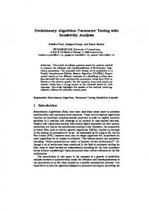
To get better insight into the best parameter ranges, we have chosen not to use the single best solution, but the 1% of the best performing parameters values during the tuning phase. Figure 1 shows the .25 and .75 quantile of those values for each of the specialists and the generalist relative to the parameter ranges. The most obvious conclusion that can be drawn from these charts, is that mutation should be low, in order to get a good performance. However, there are also some less standard conclusions. One of the most interesting results is that, although
8
Parameter Tuning of Evolutionary Algorithms: Generalist vs. Specialist
pop
toursize
pop
gengap
xover
mutprob
toursize
pop
gengap
xover
mutprob
toursize
gengap
xover
mutprob
n
n
n
(a) Generalist
(b) Ackley
(c) Griewank
pop
pop
pop
toursize
gengap
xover
mutprob
toursize
gengap
xover
mutprob
toursize
gengap
xover
mutprob
n
n
n
(d) Sphere
(e) Rastrigin
(f) Rosenbrock
Fig. 1: The good parameter ranges for each of the parameters on each test function, and the combined set. The parameter ranges from Table 2 are scaled to [0, r]
the ranges for population-size are quite different for each of the functions, the ’guesstimate’ of population-size equals 100 is not that bad after all. To be more specific, on all five problems, a population-size of 100 lies within the .25 and .75 quantile. However, most other parameter values are completely different than the ’common wisdom’ ones. For example the N parameter of N-Point crossover is much higher than 2, which indicated that uniform crossover like crossover, outperforms common 1 or 2-point crossover on these problems. This is probably due to the separable (Sphere, Rastrigin and Ackley) or partially separable nature of the test functions. Furthermore, we can observe a much higher selection pressure than normally used. Tournament sizes are almost equal to the population size, causing the evolutionary algorithm to rapidly converge towards the best individuals in the population. However, such behavior can be explained by the limited number of evaluations that the evolutionary algorithm was allowed to perform. The question rises, if such a fast-converging algorithm is always preferred over a slow-but-accurate instance. In some cases it is, while in other cases it might not be the preferred behavior. Therefore, we emphasize that the ’best parameter values’ presented here are highly related to the choices that are made in the experimental setup.
Parameter Tuning of Evolutionary Algorithms: Generalist vs. Specialist
6
9
Conclusions and Outlook
In this paper we have shown that REVAC is not only capable to find good EA parameter values for a single problem (test function), but also for a set of problems (test functions). The parameter values we found for our generalist, differ greatly from the ’common wisdom’ values that are supposed to be robust. The ‘optimal’ selection pressure for these problems, appears to be much higher than commonly used. Furthermore, a many-point crossover operator outperforms the commonly used 1 -and 2-point crossover on all five problems. On the other hand, a population-size of 100 turned out to be not that bad after all. The scope of these conclusions is limited, we do not advocate them as being the new best general parameters, because different test-suites, aggregation functions and performance measures will lead to different ‘optimal’ parameters. The best generalist will therefore always depend upon the choices that are made to define it. Based on the definition of generalist in this paper, our generalist performed quite good on most problems. However, the results on the Sphere function confirm that the no-free-lunch theorem also holds on a parameter vector level. Furthermore, the experiments revealed some major issues for parameter tuning in general. Estimating the utility has a key role in parameter tuning, both for specialists and generalists. Our experiments revealed how the number of runs per vector can influence the outcome of the experiments. Too many runs lead to high computational costs, while too few lead to an inaccurate estimated utility and therefore inaccurate results. Therefore we advocate the use of racing [2, 6, 15, 13] and sharpening [4, 13] to deal with this issue. This, on the one hand sharpens the estimate of the utility, and on the other hand reduces the computational effort. Tuning for a generalist raises specific problems. In general, it is not clear how a good generalist should be defined. In the area of multi-objective optimization several approaches are known. One approach is to use aggregation methods, like the simple average that we used here. From the results we can observe the effect of such choices; it is more effective to focus on the ’hard’ problems that can lead to high deviation in the average utility, rather than searching for a generalist that performs good on all functions. When defining tuning sessions, one have to be aware of the fact that a tuner will optimize on the problem that is defined, rather than the problem they wished to be solved. Future work can overcome this issue, by using an approach known from multi-objective optimization, namely searching for the Pareto front. Rather than aggregating the results based on choices made beforehand, such an approach allows the researcher to study the effect of a certain design choice afterwards. In [7] such an approach is used to show which parameter values are optimal, when comparing on both algorithm speed and algorithm accuracy at the same time, without specifying weights for those two objective beforehand. This approach can easily be extended to multi-function optimization, which can give insight into the the ranges of parameter-values that are most efficient on a certain problem, a class of problems, or on a whole test suite. By means of one extensive run, one can identify specialists, class-specialist, or a true generalist without defining those terms beforehand. Based on such
10
Parameter Tuning of Evolutionary Algorithms: Generalist vs. Specialist
studies, one no longer has to rely on ’common wisdom’ in order to choose their parameter values wisely but can select one that fits their needs.
References 1. Proceedings of the 2009 IEEE Congress on Evolutionary Computation, Trondheim, May 18-21 2009. IEEE Press. 2. Prasanna Balaprakash, Mauro Birattari, and Thomas St¨ utzle. Improvement strategies for the f-race algorithm: Sampling design and iterative refinement. In Hybrid Metaheuristics, pages 108–122, 2007. 3. T. Bartz-Beielstein, C.W.G. Lasarczyk, and M. Preuss. Sequential parameter optimization. In David Corne et al., editors, Proceedings of the 2005 IEEE Congress on Evolutionary Computation IEEE Congress on Evolutionary Computation, volume 1, pages 773–780 Vol.1, Edinburgh, UK, Sept. 2005. IEEE Press. 4. T. Bartz-Beielstein, K.E. Parsopoulos, and M.N. Vrahatis. Analysis of Particle Swarm Optimization Using Computational Statistics. In Chalkis, editor, Proceedings of the International Conference of Numerical Analysis and Applied Mathematics (ICNAAM 2004), pages 34–37, 2004. 5. Thomas Bartz-Beielstein and Sandor Markon. Tuning search algorithms for realworld applications: A regression tree based approach. Technical Report of the Collaborative Research Centre 531 Computational Intelligence CI-172/04, University of Dortmund, March 2004. 6. M. Birattari, T. St¨ utzle, L. Paquete, and K. Varrentrapp. A racing algorithm for configuring metaheuristics. In W.B. Langdon, editor, GECCO 2002: Proceedings of the Genetic and Evolutionary Computation Conference, pages 11–18, San Francisco CA, 2002. Morgan Kaufmann. 7. Johann Dr´eo. Using performance fronts for parameter setting of stochastic metaheuristics. In Franz Rothlauf, editor, Proceedings of the Genetic and Evolutionary Computation Conference (GECCO-2009), pages 2197–2200. ACM, 2009. 8. A.E. Eiben, R. Hinterding, and Z. Michalewicz. Parameter Control in Evolutionary Algorithms. IEEE Transactions on Evolutionary Computation, 3(2):124–141, 1999. 9. V. Nannen and A. E. Eiben. Relevance Estimation and Value Calibration of Evolutionary Algorithm Parameters. In Manuela M. Veloso, editor, Proceedings of the 20th International Joint Conference on Artificial Intelligence (IJCAI), pages 1034–1039, 2007. 10. V. Nannen and A.E. Eiben. A Method for Parameter Calibration and Relevance Estimation in Evolutionary Algorithms. In M. Keijzer, editor, Proceedings of the Genetic and Evolutionary Computation Conference (GECCO-2006), pages 183– 190. Morgan Kaufmann, San Francisco, 2006. 11. V. Nannen, S.K. Smit, and A.E. Eiben. Costs and benefits of tuning parameters of evolutionary algorithms. In G¨ unter Rudolph et al., editors, PPSN, volume 5199 of Lecture Notes in Computer Science, pages 528–538. Springer, 2008. 12. S.K. Smit. MOBAT. http://mobat.sourceforge.net, 2009. 13. S.K. Smit and A.E. Eiben. Comparing parameter tuning methods for evolutionary algorithms. In [1]. 14. David H. Wolpert and William G. Macready. No free lunch theorems for optimization. IEEE Transaction on Evolutionary Computation, 1(1):67–82, 1997. 15. B. Yuan and M. Gallagher. Combining Meta-EAs and Racing for Difficult EA Parameter Tuning Tasks. In F.G. Lobo, C.F. Lima, and Z. Michalewicz, editors, Parameter Setting in Evolutionary Algorithms, pages 121–142. Springer, 2007.