Parametric dynamic neural network recognition power - CiteSeerX

Parametric dynamic neural network recognition power B.V.Kryzhanovsky, V.M.Kryzhanovsky, A.L.Mikaelian Institute of Optical Neural Technologies, Russian Academy of Sciences 44/2 Vavilov Street, 117333 Moscow

A.Fonarev Department of Engineering Science and Physics, The College of Staten Island CUNY, SI, New York 10314

Abstract The recognition power of a network using parametric neurons is considered. Being a collection of n parametric oscillators of different frequencies and n perfect frequency filters, the neuron allows frequency parametric mixing and generation. This kind of network has the recognition power n 2 times greater than the conventional Hopfield network.

1. Introduction Today, we have the mature theory of the neural networks [1-18] based on formal McCullock-Pitts [1] neurons and designed for binary (bipolar) signal processing. Most attention is paid to formal HAM (Hopfield Associative Memory) neural net structures consisting of interconnected threshold elements – neurons [5-11]. The classic HAM model is a fully coupled neural network in which every neuron receives signals from all other neurons [5]. The interest in HAM is caused by the fact that this is the only model that allows comprehensive analysis of the net, including such aspects as the network stability, and dependence of the capacity and recognition power of associative memory on the number of neurons and interconnections [7-12, 19-26]. The possibility to build optical neural network models has been studied and some applications based on these models have been demonstrated [13-16]. The goal of the paper is to analyze the recognition power of a network that can process frequency-and-phase encoded information. The basic element of the network like that is a dynamic neuron capable of frequency generation and parametric mixing [28]. Quasi-monochromatic pulses of

n different frequencies carry the information in this network. There are some reasons to make

this kind of analysis. First, the use of optical networks implies summation of field amplitudes rather than field intensities. The approach would allow us to give up the conventional artificial adaptation of optical neural network to binary (amplitude-modulated) signals [13-17] and take full advantage

2

of optical signal processing. Second, the use of

n 2 (the effect similar to channel multiplexing) and help

number of interconnections by a factor of to overcome the




n different carrier frequencies would reduce the

problem: the number of interconnections grows as




with the number of

neurons N (in conventional neural structures the interconnection fabric takes up to 98% of the chip area). The use of high-order networks allows increased capacities of associative memory [14, 17, 18], but does not overcame the




problem. Third, it is an accepted fact that the basic elements

responsible for the high-level activity of cortex are so-called cortical columns – closely linked groups of neurons with collective properties. Theoretically, these neuron groups are capable of frequency mixing and processing of frequency-modulated signals (see references in [20-23]). However, a single neuron generates separate pulses or packets of such pulses. This fact makes neurophysiologists wonder about what kind of modulation cortical neurons use to exchange information: phase-frequency or pulse-amplitude modulation. Though the approach we discuss in the paper does not answer the question, it allows some parameters of the neural network to be evaluated for the phase-frequency coding of information signals. Note that in the paper the “parametric neuron” simulates the work of a tightly coupled neuron group (a whole cortical column) rather than a single living neuron.

2. Functioning of the dynamic neural network Consider a fully connected neural network built around

N+1

dynamic neurons in the

fashion of conventional Hopfield network [5]. Each neuron of the net is a set of parametric oscillators operating at difference frequencies. The peculiarities of functioning of such neurons proposed in [28] are given below. The aim of the net is to store and recognize a particular vector array {x(m)}. The components of the vectors are quasi-monochromatic pulses of width τ :

  



=  ω

 





+ ψ  ,

j ∈ 0, N ,

m ∈ 0, M

(1)

where ψ  is the phase resulting from interconnection travel delays and synaptic delays, and ω  is one of n fundamental frequencies of the parametric neuron oscillator (or the dynamic neuron): 



ω  ∈ ω  ω   ω  

(2)

To make the analysis more specific, we take the following conditions: τ is proportional to all characteristic oscillation periods of the neuron τ k = 2π / ω k neuron’s characteristic frequencies ωi + ω j − ω k

and τ >> τ ! ; the combination of the

is not a characteristic frequency of the neuron,

3

i.e., ωi + ω j − ω k ∉ {ω n } , except the trivial case of i = k or j = k . We assume that synaptic interconnections are also of dynamic nature and organized according to Hebb rule [2]: M

Tij = ∑ x (jm ) x (jm )*

(3)

m =0

Let us define the principle of the dynamic neuron’s function. This neuron can be regarded as a device that consists of an adder of input signals, a set of n ideal frequency filters, signal amplitude comparator, and n generators of quasi-monochromatic signals whose frequencies are determined by relation (2). The dynamic neuron works in the following way: input signals are added to give the total signal which goes to n parallel frequency filters whose outputs are compared by amplitude, the largest signal then triggers the generation of the output pulse whose frequency and phase agree with those of the initiating signal. Let us assume that the neuron has N inputs and one output and no feedback ( Tii = 0 ), and consider this algorithm of function in more detail. Signals ( X j ) that come to the i-th neuron from the other neurons are added with proper weights Tij , giving the total output signal NETi = ∑ Tij X j

j ∈ 0, N

,

(4)

j ≠i

which goes to n frequency filters of the neuron. The amplitude of the output signal of the k-th filter of the i-th neuron ( k ∈ 1, n ) is described as τ

S

(i ) k

= ∫ NETi (t − τ) exp( −iω k t ) dt / τ

(5)

0








Amplitudes 

are compared by magnitude. The following condition should be fulfilled for the 

response to be generated: if the filter of number then the neuron produces a pulse of frequency ω

= 





( 

∈



) has the maximal output signal,











in phase with







.

4

3. Recognition of a vector with phase distortion Let us assume that at the instant of time vector X whose components













=

the network under consideration receives a

are quasi-monochromatic pulses of form (1), which means that 

the i-th neuron is excited by signal 








. Let the input vector X be identical to one of the vectors

recorded in the network’s memory (e.g., X = x ( 0) ) or its distorted image: X = (θ 0 x 0(0 ) , θ1 x1( 0) ,..., θ N x N(0 ) )

(6)

where θ i is the noise caused by phase distortions in the components of the reference vector. This noise can be represented as a sequence of independent, similarly distributed random quantities: + 1, 1 − p θi =  p − 1, At time

,

≤ 

≤



,

i ∈ 0, N

(7)

= τ the signal (4) at the input of the i-th neuron will be: 

  NETi = xi(0 ) ∑ θ j + ∑ ∑ xi( m ) x (jm )* x (j0 ) xi(0)*  j ≠i m≠ 0  j ≠i 

(8)

Integrating this expression in accordance with formula (5) for the amplitudes of filtered signals, we get:   S k(i ) = xi( 0 ) δ(ω k , ω 0 i )∑ θ j + ∑ ∑ ξ (0kmij) ζ 0mij  exp[i (ω k − ω 0i )τ] j ≠i j ≠i m ≠ 0  

(9)

where δ(α,β) ≡ δαβ is the delta symbol, and ζ 0 mij = θ i exp[i(ψ mi − ψ mj + ψ 0 j − ψ 0 i )] (10) τ dt 1, ω mi − ω mj + ω0 j = ω k ξ (0kmij) = ∫ exp[i (ω mi − ω mj + ω 0 j − ω k )t ] =  τ 0, ω mi − ω mj + ω0 j ≠ ω k 0

The recognition power of this network can be analyzed by the example of a randomized array 



of vectors









stored in the network on condition that frequencies ωmj are statistically

5 

independent random quantities taking one of the values ω
ω







ω

with probability



. In

this case, the probability of quantity ξ (0kmij) taking a non-zero value is determined as:

P(ξ (0kmij) = 1) = P(ω mi = ω k ) P(ω mj = ω k ) P(ω 0 j = ω k ) + + ∑ P(ω mi = ω r ) P(ω mj = ω r ) P(ω0 j = ω k ) + r ≠k

+ ∑ P(ω mi = ω k ) P(ω mj = ω r ) P(ω 0 j = ω r ) = r ≠k

2n − 1 n3

(11)

To simplify further considerations, we assume that phases ψ mj are also independent random quantities taking 0 or π with equal probability. In this event exponent ζ µ   from (10) is a random quantity taking

±1

with probability ½ . Clear that the product

ξ (0kmij) ζ 0 mij

of two random 



quantities, one of which takes 0 and 1 and the other +1 and –1, is a random quantity η ∈ +  −

 

 

.

This way, the double sum in the right side of equation (9) should be considered as a sum of MN random independent quantities η  obeying the same distribution:  

+    η =  −  

 

− 

,

=

 

− 

 

,

r ∈ 1, MN

(12)

From what is said above and from (9) it follows that signal amplitudes after filtration are: MN N  S k(i ) = xi( 0 ) ∑ θ j + ∑ η r  1 1 

MN

S k(i ) = ∑ η r exp(iω k τ + iψ 0i )

in the channel ω k = ω 0i

(13)

in the channel ω k ≠ ω 0 i

(14)

1

For the i-th neuron to recognize the input pattern correctly, it should produce signal xi( 0 ) . As seen from (13) and (14), only the signal from the channel (13) whose frequency is equal to ω 0i can make the neuron generate the correct response (the other channels can only initiate an incorrect response of frequency other than ω 0i ). For this reason, the first necessary condition of correct recognition is

6

that quantity (13) should have the magnitude greater than any of quantities (14): in this event channel (13) suppresses the other channels (14) and gives out the output signal of correct frequency ω 0i . The second necessary condition is that the quantity in the square brackets (13) should be greater than zero: in this case the phase of the output signal agrees with the phase of xi( 0) . Otherwise recognition failure occurs. We see that the probability of recognition failure for a particular component can be written as N  MN  Pi = P ∑ η r ≥ ∑ θ j  1 1 

(15)

In view of [19,24-26], we use Chebyshev-Chernov method [27] to determine the upper limit of recognition failure probability (15). According to the method, we have the following relation for any
≥ : MN N   MN N   P ∑ θ j ≤ ∑ η r  ≤ exp  z  ∑ η r − ∑ θ j  = 1 1 1     1

 

= (   η



) (   −

 

θ

)



=

    −              −    = + + −  + − 

[

] [

]

(16)

where the bar stands for averaging over ensembles (7) and (12). Then we minimize expression (16) with respect to  ≥  . Note that this expression as a function of z is convex downwards. By differentiating with respect to z and putting the derivative to zero, we find that its minimum is at z meeting the equation: pq( M + 1)e 4 z + p (1 − 2q )e 3 z + q(1 − p )(M − 1)e 2 z − − (1 − p)(1 − 2q )e z − q (1 − p )(M + 1) = 0

(17)

What should be done next is to determine the root of the equation and substitute it in (16). In the most interesting case of



 −



>>



the root of (17) can be expressed as a power series function of

. Substituting the corresponding expression in (16) and considering only the leading terms of

the series for



>>  , we get for the probability of vector recognition failure:

7



≤







 −   


 −   



(18)

The resulting inequality sets the upper limit for the mean error probability in the network with parameters ( N ; M ; n ; p) . With growing N, this limit approaches zero each time when M, as a function of N, grows slower than 

=



 

   −   

 

(19)

In view of [8-11] this gives us grounds to regard quantity (19) as the associative memory power that the neural network under consideration can asymptotically attain.

4. Recognition of vectors with frequency distortions. This paragraph deals with a more complicated case when the distortions of the input vector are caused by two simultaneous processes: distortions in signal phase and frequency. This statement of problem corresponds to the input vector of the following form: θ j = θ (jψ ) θ (jω) ,

X = (θ 0 x 0(0 ) , θ1 x1( 0 ) ,..., θ N x N(0) ) ,

j ∈ 0, N

(20)

where θ (ψj ) is the phase-distortion multiplicative noise component that we considered in the previous paragraph; θ (ωj ) is the frequency-distortion multiplicative noise component. The intensity of the noise components is a sequence of independent similarly distributed random quantities: + 1, 1 − p θ (jψ ) =  p − 1,

(21)

1, 1 − pω  θ (jω) =  pω exp[i(ων − ω0 j )t ] ,

(22)

and

where





≤ ≤  ,



≤

ω

≤

!

'

(

, ω ν ∈ ω* # ω ) #%$&$&$ # ω " . Here the probability that frequency ω ν and

frequency ω0 j are the same (no frequency distortion) is 1 − p ω and that they are not is +

ω

.

Substituting (20) in (5) and making necessary mathematical manipulations, we find the signals leaving the filtering channels of the i-th neuron to be:

8

MN N  S k(i ) = xi( 0 ) ∑ ξ j + ∑ η r  1 1 

(23)

MN N  S k(i ) = ∑ ζ j + ∑ η r  exp(iω k τ + iψ 0 i ) 1 1 

(24)

in the channel ω k = ω 0 i ;

in the channel ω k ≠ ω 0i . Here η r is defined by expression (12), and random quantities ξ j and ζ j are determined as:  + 1, (1 − p)(1 − p ω )  ξ j =  0, , pω  −1 p (1 − p ω ) 

 + 1,  ζ j =  0,  −1 

p ω (1 − p) / n 2 1 − ( pω / n 2 ) pω p / n 2

(25)

To calculate the probability of recognition failure for component xi( 0) , let us apply the method we used for obtaining expressions (16-18). First we perform averaging over statistical distributions (12) and (25), and then minimize the resulting expression. Let a non-negative parameter z be the root of the following equation: p( M + 1)e 4 z + (MR + pQ)e 3 z + (1 − 2 p)( M − 1)e 2 z − − [ MR + (1 − p )Q]e z − (1 − p)(M + 1) = 0

(26)

where Q ≡ (1 − 2q) / q and R ≡ pω /(1 − pω ) . Then the expression for the upper limit of recognition failure probability can be written as: P ≤ Ne − NC

(27)

C = z ( M + 1) − M ln[ q(e 2 z + Qe z + 1)] − ln[(1 − pω )( pe 2 z + Re z + 1 − p)]

(28)

where

For the asymptotic limit N → ∞ , M >> 1 , expressions (27-28) become much simpler. In particular, expanding (28) into a series with respect to small parameter M −1 , we find that

9

(1 − 2 p) 2 (1 − p ω ) 2 C≈ 4qM

(29)

 (1 − 2 p ) 2 (1 − p ω ) 2  P ≤ N exp − N  4qM  

(30)

and the recognition failure probability

We see that this expression agrees with (18) to factor (1 − pω ) 2 .

5. Analysis Assuming that ω =




for all

Hopfield network. Indeed, in this event



∈







(Q=0 and R=0) and the components of all memory

∈ + − . Accordingly, expressions (27-30) change into the 





, we come to the well-known case of the bipolar 

= 



vectors take only two values









known formulae (see [8-11, 18, 19-26] and references therein). The study we made above is of interest when replaced by 





≥ . In this event quantity 



− 

can be

to good enough accuracy. Then (30) can be rewritten as:  (1 − 2 p) 2 (1 − pω ) 2  P ≤ N exp − Nn 2  4M  

(31)

Correspondingly, the asymptotically achievable power of associative memory of the network under consideration takes the form: (1 − 2 p ) 2 (1 − p ω ) 2 M = Nn 4 ln N 2

(32)

As follows from (30-32), the neural network is more susceptible to phase jitter, while the effect of frequency distortions on the recognition process is less pronounced. As the number n of carrier frequencies goes up, the noise immunity of the associative memory under consideration increases noticeably. So does its memory capacity, which is 



times greater than that of

conventional Hopfield network. Besides, unlike Hopfield network, the number M of patterns this kind of network can store can be many times greater than the number of neurons N. These properties are caused by the fairly complicated structure of the dynamic neuron the network uses.

10

Indeed, that the dynamic neuron has filtering channels leads to suppression of most noise components that result from parametric frequency mixing at the neuron input. The noise falls in each channel, which is clearly seen in the probability distributions (12) and (25).

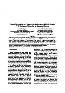
t=0

t = 20

t = 40

t = 60

t = 80

t = 100

Fig.1. Pattern recognition process at N=100, M=200, n=15, p=0.2, pω = 0 . For example Fig.1 shows pattern recognition by network constructed of 100 parametric neurons: 200 randomized patterns are stored in the network; 20% of input vector components are phase-distorted and the frequency-distortion is neglected; dynamic neurons possess 15 natural frequencies. The states of network processing data in asynchronous regime are shown at every 20 tact (t=0, t =20, ..., t =100) of recognition process. It is obvious that the recognition fulfilled successively in spite of M > N . In conclusion we can say that: a) introduction of frequency characteristics for input pattern components results in the considerable increase of the network memory capacity and higher recognition efficiency; b) due to “multiplexing” we can decrease the number of interconnections by


times without having to reduce the memory capacity and recognition efficiency, thus solving the N 2 problem to some extent; c) it is essential that the memory capacity may be varied at a constant

number N, i.e. without variation of stored vector’s dimension. Of course, the sophisticated design of the neuron results in the increased number of its intrinsic interconnections. However, the fact that the neuron has fewer long-distance interconnections with other neurons is more important.

11

The study was supported in part by the Russian Foundation for Basic Research (project 0107-90308) and RAS program “Intellectual Control Systems” (project 4.5).

References [1]. W.S.McCulloch and W.Pitts, "A logical calculus of the ideas imminant in nervous activity", Bull.Math.Biophys., vol.5, pp.115-133, 1943. [2]. D.O.Hebb, The Organization of Behavior. New York:: Wiley, 1949. [3]. D.J.Willshaw et al, "Non-holographic associative memory", Nature, vol.222, pp.960-962, 1969. [4]. T.Kohonen, Self-Organization and Associative Memory. Berlin: Springer-Verlag, 1984. [5]. J.J.Hopfield, “Neural networks and physical systems with emergent collective computation abilities”, Proc.Nat.Acad.Sci.USA, vol.79, pp.2554-2558, 1982. [6]. D.W.Tank and J.J.Hopfield, "Simple neural optimization network", IEEE Trans.Circuits Syst., , vol. CAS-33, pp.533-541, 1986. [7]. G.E.Hilton and J.A.Andersen, "Parallel models of associative memory". Hillsdale, NJ:Erlbaum, 1981. [8]. R.J.McEllise, E.C.Posner et al. , “The capacity of Hopfield associative memory”, IEEE Trans. Inf. Theory, 33, pp. 461-482 (1987). [9]. W.A.Little and G.L.Shaw, "Analytic study of the memory storage capacity of a neural network", Math.Biosci., vol.39, pp.281-290, 1978. [10]. H.J.Sussman, “On the number of memories thet can be stored in a neural nets with Hebbs weights”, IEEE Trans. Inf. Theory, 35, pp.174-178 (1989). [11]. A.Kuh and B.W.Dickson. “Information capacity of Associative Menory“, IEEE Trans. Inf. Theory, vol. 35, pp.59-68 (1989). [12]. L.Wang, , “Effects of noise in training patterns on the memory capacity of the fulli connected binary Hopfield neural network”, IEEE Trans. of Neur. Netw., 9, pp.697-704 (1998). [13]. D.Psaltis and Y.S.Abu-Mustafa, "Computation power of parallelism in optical computer", Dep.Elec.Eng., Calif.Inst.Tech., Pasadena, preprint, 1985. [14]. B.S.Kiselev, N.V.Kulakov, A.L.Mikaelian, and V.A.Shkitin, “Optical implementation of highorder associative memory”, Intern.Journ.of Optical Computing, vol.1, pp.89-92, 1990. [15]. B.S.Kiselev, N.V.Kulakov, A.L.Mikaelian, and V.A.Shkitin, “Optical auto- and heteroassociative memory for strongly correlated patterns”, Radiotechnika, vol.4, No.3, pp.80-90, 1992.

12

[16]. V.A.Ivanov, B.S.Kiselev, A.L.Mikaelian, and D.E.Okonov, “Optoelectronic neuroproce ssor based on holographic disc memory using 1-D hologramm recording”, Optical Memory and Neural Networks, vol.1, No.1, pp.55-62, 1992. [17]. B.S.Kiselev, N.V.Kulakov, A.L.Mikaelian, and V.A.Shkitin, “Optical high -order associative memory using neural networks ”, Radiotekhnika, Vol.10, pp.54 -62, 1990. [18]. D.Burshtein. “Long -Term Attraction in Higher Order Neural Networks”, IEEE Trans. of Neur. Netw., vol. 9, N4, pp.42-50 (1998). [19]. B.V.Kryzhanovsky, V.N.Koshelev, A.L.Mikaelian and A. Fonarev. “Recognati on Ability of


      "! #$&%'() *
(+, -/.10 234
1  657 $ 85 9 :6;

-276 (2000).

[20]. P.A.Annios, B.Beek, T.J.Csermely and E.M.Harth. "Dynamics of neural structures", J.Theor.Biol., vol. 26, pp.121-148, 1970. [21]. M.Usher, H.G.Schuster and E.Neibur. "Dynamics of population of integrate-and-fire neurons, partial sinchronization and memory", Neural Computation, vol.5, pp.370-386, 1993. [22]. N.Farhat. “Corticonics: the way to designing mashines with brain -like intelligence”, SPIE’2000, pp. 158-170, San-Diego, 2000. [23]. F.C.Hoppensteadt, E.M.Izhikevich. “Pattern recognition via synchronization in phase -locked loop neural networks”. IEEE Trasactions on Neural Networks, vol.11, N3, pp.734 -738 (2000). [24]. B.V.Kryzhanovsky, V.N.Koshelev. A.Fonarev. “Estimating efficiency of randomized Hopfield memory”. Problemi Peredachi Informacii, vol. 37, N.2, pp.77-87 (2001) [25]. A.Fonarev, B.V.Kryzhanovsky, M.V.Kryzhanovsky, V.N.Koshelev. “Adaptation of Hopfield associative memory parameters in statistic training”. Optical Memory&Neural Network, Vol. 10,

? @6ABBDC EGF -98 (2001).

[26]. A.Fonarev, B.V.Kryzhanovsky. “On optimization of neural network recognition capability”.

H'I(J)KLMN(O,PQ-RS/T1UVPW3S4MN1VPJXRS Y6Z[ RN\D]^Z-_ `a6bdc6eeGfhghi

[27]. N. Chernov, “A mesure of asimptotic e fficiency for tests of hupothesis besed on the sum of observations”, Ann. Math. Statistics, vol.23, pp.493 -507 (1952). [28]. B.V.Kryzhanovsky, A.L.Mikaelian. “On recognation ability of neuronet based on neurons with parametrical frequencies conversion”. Do kladi Akademii Nauk, vol.

j6k&jlmnjlooDpq -4 (2002).