Parametric Stabilization of Automatic Control Systems - Springer Link

ISSN 0005-1179, Automation and Remote Control, 2011, Vol. 72, No. 11, pp. 2300–2314. © Pleiades Publishing, Ltd., 2011. Original Russian Text © V.A. Kamenetskii, 2011, published in Avtomatika i Telemekhanika, 2011, No. 11, pp. 86–101.

DETERMINATE SYSTEMS

Parametric Stabilization of Automatic Control Systems V. A. Kamenetskii Trapeznikov Institute of Control Sciences, Russian Academy of Sciences, Moscow, Russia Received June 6, 2011

Abstract—A method for selection of the stabilizing parameters was proposed for the control system closed by a unit with saturation. It was intended for designing the closed-loop control systems meeting a number of requirements on the transient performance. Apart from the asymptotic equilibrium stability, it is required that the attraction domain must include a prescribed set of initial deviations and the solutions beginning in this set should remain in the permissible set and have a certain degree of damping. DOI: 10.1134/S0005117911110051

1. INTRODUCTION By the parametric stabilization is meant [1, 2] determination of the values of parameters on which the right side of the system in deviations depends so that the closed-loop system becomes stable and satisfies the requirements on the transient performance and, in particular, on the attraction domain. The parameters are determined in advance prior to activating the system and without using the adaptation mode. As applied to the automatic control systems, this implies that the controller structure is assumed to be given and the controller parameters play the role of the unknown stabilizing parameters to be determined or adjusted. Letov in [3] noted that “. . . in the problem of design the practical significance of the attraction domain is immense” and formulated a promising problem of “. . . constructing the attraction domain for any case of closure.” The present paper follows another approach: determine the requirements to be satisfied by the closed-loop system and then seek purposefully the controller parameters for which the closed-loop system meets these requirements. Apart from ensuring the asymptotic stability of equilibrium, we confine here our consideration to three requirements on the choice of controller. (1) The attraction domain of the closed-loop system must contain the desired (meeting the designer’s interests) set of the initial deviations H0 , that is, the solutions beginning at H0 must tend to equilibrium. (2) The solutions beginning in the set H0 should not leave the given permissible set A (in particular, this counteracts the overshoot). The set A is defined by the phase constraints and has the sense of the domain of safe system operation. By defining the set A, the overshoot effect may be constrained only along certain directions, which seems very convenient from the application standpoint. (3) The solutions beginning in the set H0 must have a certain—as great as possible—exponential degree of damping. It is how provision of speed for the selected set of solutions is understood. It is paradoxical, but in the context of the overshoot problem a greater attraction domain of the closed-loop system is not a blessing. Let it be required to drive the system from the set H0 to the origin without leaving the set A of safe system operation. A great attraction domain S such that A ⊂ S is not sufficient for that. It is necessary to know an invariant estimate Sest ⊂ S such that H0 ⊂ Sest ⊂ A, and at closing the system’s loop, determination of such estimate comes to the foreground. The above requirements on the transient performance almost completely repeat the 2300

PARAMETRIC STABILIZATION OF AUTOMATIC CONTROL SYSTEMS

2301

similar requirements in [3] (but not their content). The requirement of H0 ⊂ S at selection of the feedback was proposed in [4]. The question of the size of the set H0 was related in [5] with the value of the control resource. The requirement H0 ⊂ Sest ⊂ A is used in [1, 2]. It seems that for the first time all three requirements were formulated as a triunity in [6, 7]. It is understandable that the degree of success in satisfying the aforementioned requirements depends on the control system characteristics and the accepted trade-off between the requirements. It must be stressed that the popular methods of selecting the controller parameter such as the modal control and analytical design of the optimal controllers (ADOP) [8, 9] are not oriented to rendering the aforementioned properties to the closed-loop system. The present paper assumes that the controller is defined by the saturation function (saturator) of the generally nonlinear smooth function depending on the parameters. The case of adjusting a smooth controller goes in [1]. 2. FORMULATION OF THE PROBLEM The nonlinear stationary control system with additive scalar control obeying in a certain domain G ⊂ Rn the differential equations x˙ = f1 (x) + uf2 (x),

(1)

where x ∈ Rn is the vector of phase variables and fi (x) ∈ C (2) (G → Rn ), i = 1, 2, is considered as the control plant. It is assumed that the control in the form of the feedback function u = u(x) satisfies the constraint |u(x)|  1

(2)

and, using some of the earlier methods, was already selected as the saturation function (saturator) with the nonlinear switching function c(α1 , x): 

u(x) = sat(c(α1 , x)) =

c(α1 , x), |c(α1 , x)| < 1 sgn(c(α1 , x)), |c(α1 , x)|  1,

where α1 ∈ U1 ⊂ RN1 is the parameter vector and c(α1 , x) ∈ C (2) (U1 × G → R). Therefore, the subject matter is represented by the control system x˙ = f1 (x) + sat(c(α1 , x))f2 (x),

(3)

where the stabilizing parameters α1 are to be determined. It is assumed that for α1 ∈ U1 system (3) is asymptotically stable in zero and the set Ec (α1 ) = {x ∈ Rn : |c(α1 , x)|  1}

(4)

includes the origin. Let the permissible domain defined by the phase constraints be given by the nonlinear inequality Ad = {x ∈ G ⊆ Rn : g(α1 , x) < 0},

(5)

where g(α1 , x) ∈ C (2) (U1 × G). We assume that the parameter defining the constraints is united formally with the system parameter. The case of more than one smooth constraint (they are equivalent to one nonsmooth constraint, their maximum) is not a fundamental obstacle, but hinders the presentation and is omitted here. AUTOMATION AND REMOTE CONTROL

Vol. 72

No. 11

2011

2302

KAMENETSKII

Let H0 ⊂ Rn be the set of initial deviations to be included in the attraction domain of the closed-loop system. For simplicity we assume that H0 is given by 



H0 = μ co aj , j = 1, J , ,

(6)

where aj ∈ Rn are the vertices of a convex polyhedron H0 , μ > 0 is the parameter enabling one to increase and decrease proportionally H0 (co{ · } denotes the convex hull of the set { · }). In the case of arbitrary H0 it can be embedded in a polyhedron like (6). Of independent interest is also a linear variant of system (3), namely, the stationary linear control system closed by a linear saturator x˙ = Ax + b sat( c, x n ),

(7)

where x(t) ∈ Rn is the vector of phase variables, A is the given constant real (n × n) matrix, b ∈ Rn is the given constant vector, the pair (A, b) is stabilizable ( · , · m denotes the scalar product in Rm ). By the linear saturator is meant the saturation function of the linear function of coordinates 

u(x) = sat( c, x n ) =

 c, x n , | c, x n | < 1 sgn( c, x n ), | c, x n |  1.

(8)

Here the vector c is a smooth function of the parameter α1 , that is, c = c(α1 ) ∈ C (2) (U1 → Rn ). In the most commonly encountered special case, the vector c is considered as the parameter vector (c = α1 , N1 = n). In this case, the coefficients of the linear function  c, x n play the role of unknown stabilizing parameters c = α1 ∈ U1 to be determined. It is assumed that for α1 ∈ U1 the matrix Ac = A + bc (α1 ) is asymptotically stable ((·) stands for transposition), that is, Re(λi (Ac )) < 0, i = 1, n, which makes system (7) asymptotically stable in the small. Despite the seeming simplicity of system (7), the study of its stability in large or, stated differently, the study of its attraction domain is a challenge. This is explained by the fact that, first, system (7) is nonlinear and, second, the right-hand side of system (7) is a sectionally continuous function, which gives rise to the need for dividing the system’s phase space into three smoothness domains of the right-hand side. One of them, the linearity domain of system (7), is as follows: Ec = {x ∈ Rn : | c, x |  1} . The set

(9)



Uc =

     Ac t x ∈ R : max  c, e x   1 n

(10)

0t 0, which makes negative the second term in (12). For (13), the inequality v(x, ˙ u∗ (x)) < 0, x = 0 passes into the inequality ∂v(x)/∂x, f1 (x)n − k ∂v(x)/∂x, f2 (x)2n < 0,

x = 0.

(14)

It remains to indicate a definite positive Lyapunov function v(x) satisfying (14), and the problem of stabilization is solved. If now a linear system (with f1 (x) = Ax and f2 (x) = b) is taken as (1) AUTOMATION AND REMOTE CONTROL

Vol. 72

No. 11

2011

2304

KAMENETSKII

and the quadratic form v(x) = x Lx, where L = L is a symmetrical matrix, as the Lyapunov function, then control (13) goes over to u∗ (x) = −2k Lb, xn and the relation (14) becomes for k = 1/2R and Q = Q > 0 the Riccati equation A L + LA − (1/R)Lbb L = −Q,

(15)

corresponding to minimization of the quadratic functional ∞

(x Qx + v  Rv)dt.

J = 1/2

(16)

0

If the control is subject to constraint (2), it is proposed in [8] to take the saturator (8) with c = −(1/R)Lb, that is, u∗ (x) = −sat( (1/R)Lb, x n )

(17)

as the optimal design for the functional (16). For the initial points from the set of linear stabilization Uc from (10) for c = −(1/R)Lb, this control is, obviously, optimal for functional (16). Optimality of control (17) for the initial point beyond the set Uc requires a special study, and, therefore, we omit the details and just note the paper [10]. 4. MAIN RESULT: METHOD TO DETERMINE THE CONTROLLER PARAMETERS To determine the controller parameters, the present paper uses a modification of the algorithm from [1]. The desired invariant estimate of the attraction domain is bounded by the level surface of some Lyapunov function. By considering the Lyapunov function from the parametric class and the system as depending on the parameters, we get the problem of determining a totality of unknown parameters. The differential algorithm of variation of the totality of parameters [1] allows one to increase the desired invariant estimate in certain directions. It is assumed that at the initial stage the values of parameters corresponding to some initial estimate and playing the role of initial conditions for the differential algorithm are known. The algorithm of [1] was developed for the closed-loop systems having parameter in the normal Cauchy form x˙ = f (α2 , x),

f (α2 , 0) = 0,

α2 ∈ U2 ⊆ RN2 ,

(18)

where x ∈ G ⊂ Rn is the vector of phase coordinates, α2 ∈ U2 ⊆ RN2 is the vector of parameters, the function f (α2 , x) ∈ C (2) (U2 × G), and G ⊆ Rn is some domain. System (3) and its linear variant (7) can be well regarded as systems like (18) with the only stipulation that the right-hand side of system (3) is not a smooth function. We introduce the vector α = (α1 , α2 ) ∈ U1 ×U2 ⊆ RN , N = N1 +N2 , uniting the system parameters and those of the Lyapunov function. In what follows, for system (3) we use its representation in the form (18) for f (α, x) = f1 (x) + sat(c(α1 , x))f2 (x). According to [1], to allow for the phase constraints like (5) one need the function M (α, x) = max{vλ (α, x), g(α, x)},

(19)

where the ordinary derivative of the Lyapunov function v(α, ˙ x) =  ∂v(x)/∂x, f (α, x) n is replaced ˙ x) + 2λv(α, x) in order to ensure the desired rate of decrease. by vλ (α, x) = v(α, AUTOMATION AND REMOTE CONTROL

Vol. 72

No. 11

2011

PARAMETRIC STABILIZATION OF AUTOMATIC CONTROL SYSTEMS

2305

Definition. By the domain of λ-attenuation of system (18) we mean the set S(α, r) depending on the parameters α and r > 0 and featuring the following characteristics: (1) the set S(α, r) is a connected component of the set G(α, r) = {x ∈ Rn : 0 < v(α2 , x) < r} ∪ {x = 0} including the point x = 0; (2) U ∗ (0) ⊂ S(α, r) ⊂ Hα , where U ∗ (0) ⊂ Rn is a neighborhood of the point x = 0 and Hα ⊂ G ⊂ Rn is a compact; (3) the inclusion S(α, r) ⊆ D(α) = {x ∈ Rn : M (α, x) < 0} ∪ {x = 0} is satisfied. The so-defined domain S(α, r) has all properties of the attraction domain such as asymptotic stability of the origin, attraction, that is, it follows from x0 ∈ S(α, r) that x(x0 , t) → 0, t → ∞, and invariance, that is, it follows from x0 ∈ S(α, r) that x(x0 , t) ∈ S(α, r) for t  t0 . Additionally, the domain of λ-attenuation is contained in the permissible domain S(α, r) ⊆ Ad (the phase constraint g(α, x) < 0, and the condition for the derivative of the Lyapunov function vλ (α, x) < 0 enjoys equal rights in determination of the domain S(α, r)). It follows from definition that for x(t0 ) ∈ S(α, r) along any solution of system (3) valid is the exponential estimate of attenuation of the Lyapunov function v0 (x(t))  e−2λ(t−t0 ) v(x(t0 )) which in the case of Lyapunov functions from the class of uniform even-degree forms entails exponential decrease of the norm of solution of system (3). We denote by R(α) the critical value of the level constant for which condition (3) of definition is violated, that is, the set S(α, R(α)) is the best domain of λ-attenuation for a fixed Lyapunov function. We denote by I(α) the set of the tangency points of the sets bnd(S(α, R(α))) and B(α), where B(α) = bnd(Dc (α)) H (bnd( · ) denotes the domain boundary) and Dc (α) is a connected component of the set D(α) including x = 0, compact H from Condition 1. To determine the value of α for which the inclusion H0 ⊂ S(α, R(α)) exists for the greatest μ, it is suggested to vary the parameter α along the solutions of the differential inclusion α(t) ˙ ∈ F (α(t)).

(20)

The multivalued map F (α) : Rn → P (Rn ), where P (Rn ) is the set of all subsets Rn , is selected so that the relations [1] λj (α(t1 ))aj ∈ S(α(t2 ), R(α(t2 ))),

t1 < t2 ,

j = 1, J ,

(21)

where the vectors aj , j = 1, J , define the set H0 from (6) and the vectors yj = λj (α)aj , j = 1, J , are determined from the condition yj ∈ bndS(α, R(α)), are satisfied at variation of the vector α = α(t) along solution (20). For the convex S(α, R(α)), satisfaction of (21) provides increase of the greatest value of μ for which the polyhedron H0 ⊆ S(α, R(α)). The function M (α, x) from (19) is nondifferentiable because of the phase constraints (as on M (α, x) from [1]) and the presence of a saturator. To avoid bulky discussions, we confine ourselves to the case characterized by satisfaction of the following condition. Condition 0. The inequalities | c(α1 , x) |= 1 and vλ (α, x) − g(α, x) = 0 are satisfied for all x ∈ H such that M (α, x) = 0 (compact H from Condition 1). Condition 0 implies that, for those α for which it is satisfied, the function M (α, x) is twice continuously differentiable in the neighborhood of the points x ∈ H such that M (α, x) = 0, the requirement on smoothness of the functions f1 (x), f2 (x), and c(α1 , x) being included in the definition of system (3). The following conditions repeat those of [1]. AUTOMATION AND REMOTE CONTROL

Vol. 72

No. 11

2011

2306

KAMENETSKII

Condition 1. There are neighborhood U ∗ (0) ⊂ Rn and compact H ⊂ Rn such that U ∗ (0) ⊂ S(α, R(α)) ⊂ H. Condition 2. ∂M (α, x)/∂x = 0 for all x ∈ H such that M (α, x) = 0 and x = 0. Condition 3. For all x ∈ I(α) on the vectors h = 0 for which ∂M (α, x)/∂x, h n = 0, valid is the inequality 



∂ 2 M (α, x) ∂ 2 v(α, x) − γ(α, x) h, h ∂x2 ∂x2

> 0, n

where the coefficients γ(α, x) > 0 obey the relations ∂v(α, x)/∂x = γ(α, x) (∂M (α, x)/∂x) following from the necessary conditions for local minimum of the extremal problem R(α) = min v(α, x).

(22)

x∈B(α)

It is clear that Conditions 2 and 3 make sense only for those α for which Condition 0 is satisfied. Condition 4. The value of R(α) is defined as the solution of problem (22), and the equality I(α) = Argmin v(α, x) x∈B(α)

holds for the set I(α). Condition 5. ∂v(α, x)/∂x = 0 for x ∈ bndS(α, R(α)). We consider the multivalued map F : α → P (Rn ) such that the set F (α) consists of the vectors w ∈ RN satisfying for all x ∈ I(α) and yj = λj (α)aj , j = 1, J , the relations 



∂M (α, x) ∂v(α, yj ) ∂v(α, x) − + γ(α, x) ,w ∂α ∂α ∂α



 −ε(α),

(23)

N

where the coefficients γ(α, x) > 0 follow Condition 3 and ε(α) > 0 is a continuous function. Theorem 3 from [1] stating that if there exists a neighborhood U ⊂ RN such that for all α ∈ U satisfied are Conditions 0–5, S(α, R(α)) = ∅, and F (α) = ∅, then relation (21) is valid for the differential algorithm (20) for F (α) = F (α) along solutions α(t) ∈ U . Unfortunately, for a wide range of problems the parameters of the controller α1 along solutions of (20) for F (α) = F (α) do not vary reasonably. Such problems include stabilization of the linear system (7) with the use of quadratic Lyapunov functions for λ = 0 and without phase constraints. Indeed, it was shown in [11] / Ec follows from x ∈ I(α). Consequently, that for this case B(α) Ec = ∅ (Ec from (9)) and x ∈ the right-hand side of system (7) is independent of the vector c at the points x ∈ I(α). Therefore, inequalities (23) defining the multivalued map F (α) are independent of the vector c (hence of α1 ), and the parameter α1 along the solution of (20) may vary arbitrarily, if at all, as long as the aforementioned conditions for algorithm’s operation are not violated. One of the causes of this violation is the violation of inequality M (α, x) < 0 inside S(α, R(α)) which is due either to growth of the local maxima of the function M (α, x) within S(α, R(α)) or violation of the negative definiteness of M (α, x) at the point x = 0, M (α, 0) = 0 being already a local maximum. Publications to appear soon present a modification of algorithm (20) oriented to retaining the negativeness of M (α, x) within S(α, R(α)) for the general case of system (3) and arbitrary parametric class of the Lyapunov functions. Here, we confine ourselves to a theorem establishing the lack of the local maxima M (α, x) (except for x = 0) within S(α, R(α)) in the case of the linear system (7) and the Lyapunov functions from the parametric class of homogeneous forms of an arbitrary even degree. AUTOMATION AND REMOTE CONTROL

Vol. 72

No. 11

2011

PARAMETRIC STABILIZATION OF AUTOMATIC CONTROL SYSTEMS

2307

We proceed to a modification of algorithm (20) retaining along its solutions the negative definiteness of M (α, x) at the point x = 0 and assume that in the neighborhood of zero M (α, x) = vλ (α, x). Condition 6. The negative definiteness of M (α, x) in the neighborhood of zero is defined by the negative definiteness of some homogeneous even-degree form v2d (α, x) depending linearly on the parameter α. We take the function λ(α) = max v2d (α, x)

(24)

x=1

as the characteristic of retaining the negative definiteness of v2d (α, x). The function λ(α) of (24) is convex and continuous and, consequently [18], local-Lipschitzian. Therefore, its generalized Clark gradient coincides with the subdifferential in the convex-analytical sense and obeys the expression [18] 

∂λ(α) = co



∂v2d (α, x) , v2d (α, x) = λ(α), x = 1 . ∂α

(25)

Let λ0 > 0 be some constant. Along with λ(α), we consider the function

λ(α) = max{λ(α), −λ0 }.

(26)



of the function λ(α), valid is the representation [18] For the generalized Clark gradient ∂ λ(α)

= ∂ λ(α)

⎧ ⎪ ⎨ ∂λ(α)

if λ(α) > −λ0 co {0, ∂(λ(α))} if λ(α) = −λ0 ⎪ ⎩ 0 if λ(α) < −λ0 ,

the function λ(α) being regular [18]. We define the multivalued map F2d (α) by the relations 



. F2d (α) = y ∈ RN : y, xN  0, x ∈ ∂ λ(α)

(27)

Modification of algorithm (20) lies in imposing additional constraints on the right-hand side of (20). Namely, F (α) is defined by F (α) = F (α)



F2d (α),

(28)

where the maps F (α) and F2d (α) are defined in (23) and (27), respectively. In this case, algorithm (20) has in addition to (21) the properties concerning retention of the sign of the Lyapunov function derivative. We denote by dom(F ) the set of α such that for them S(α, R(α)) = ∅ and F = ∅, and by int( · ) the interior of the set ( · ). Theorem 1. Let for some λ0 > 0 dom(F ) = ∅, and there be a neighborhood U ⊆ dom(F ) / ∂λ(α) for such that Conditions 0–6 are satisfied for all α ∈ U and also int(F (α)) = ∅ and 0 ∈

λ(α) = λ(α), where the generalized Clark gradient of the function λ(α) of (24) is defined in (25). Then, for any point α0 ∈ U ⊆ dom(F ) there exists a continuously differentiable solution α(t) (α(0) = α0 ) of inclusion (20) with F (α) from (28). Any such solution satisfies (21) for [t1 , t2 ] ⊆

from (26) satisfies the inequality [0, T ], and the function λ(α)



λ(α(t 1 ))  λ(α(t2 )),

t1 < t2 ,

where [0, T ] is the existence interval of the solution. AUTOMATION AND REMOTE CONTROL

Vol. 72

No. 11

2011

(29)

2308

KAMENETSKII

Theorem 1 is proved in the Appendix.

The constant λ0 and function λ(α) from (26) play the following roles. Under the conditions of Theorem 1, the set I(α) of the tangency points of the surfaces M (α, x) = 0 and v(α, x) = R(α) is finite. Relation (23) defining F (α) represents a system of algebraic linear inequalities relative to the vector w. The number of these inequalities is defined by the number of points in I(α) and the number J of vectors aj . The set F2d (α) is also defined by the system of linear inequalities (27). Correspondingly, F (α) = F (α) F2d (α) is defined by the inequalities uniting (23) and (27). If this united system has no solutions, that is, F (α) = ∅, then the algorithm is aborted. Reduction in λ0 leads to F2d (α) = Rn , that is, F (α) is defined only by (23). Therefore, the number of inequalities in the united system is decreased, thus facilitating its solvability. Now we demonstrate how Theorem 1 is simplified in the case of the linear system (7) and the Lyapunov functions from the parametric class Φ2p of homogeneous forms of degree 2p, that is, functions of the form v(α2 , x) =

N2 

αi2 ϕi (x) = α2 , ϕ(x)N2 ,

ϕi (x) = xi11 . . . xinn ,

i=1

n 

ij = 2p,

j=1

where x ∈ Rn , α2 ∈ RN2 is a set of uncertain coefficients of the Lyapunov function and ϕ(x) = (ϕ1 (x), . . . , ϕN2 (x)) is a set of monomials of the specified form. The following theorem reflects the specificity of algorithm (20) at using the Lyapunov functions of the class Φ2 p for the linear systems like (7). Theorem 2. Let in the case of (7) and v(α, x) ∈ Φ2 p the set S(α, R(α)) = ∅ for α ∈ U . Then, the following assertions are valid for α ∈ U : (1) Condition 5 of Theorem 1 is satisfied mechanically. (2) Conditions 0 and 2 of Theorem 1 are satisfied if there are no phase constraints, that is, Ad = Rn and M (α, x) = vλ (α, x). (3) If for α ∈ U the function g(α, x) has no local maxima in H, then the set S(α, R(α)) has no local maxima of the function M (α, x), except for x = 0, S denoting closure of the set S . (4) 0 ∈ / ∂λ(α). (5) int F2d (α) = ∅. Theorem 2 is proved in the Appendix. 5. EXAMPLES To illustrate the results obtained, we consider numerical examples of the second-order control systems both linear like (7) (Examples 1 and 2) and nonlinear like (3) (Example 3). We use the Lyapunov functions from the parametric classes of homogeneous forms of the second and fourth orders, as well as from the parametric class of the third-degree polynomials which has no linear monomials. The following results were obtained using algorithm (20) for various combinations of the directions of increase of the domains of λ–attenuation. Example 1 [14]. We consider the system x˙1 = x2 ,

x˙2 = u,

u = sat( c, x )

(30)

representing the double integrator closed by a linear saturator. The parameters ci for system (30) are selected in [14] so as to provide the best estimate of the attraction domain of the closed-loop system with regard for the phase constraints g(x) = x22 − 1 < 0 AUTOMATION AND REMOTE CONTROL

(31) Vol. 72

No. 11

2011

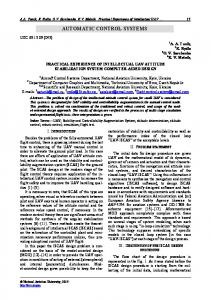
PARAMETRIC STABILIZATION OF AUTOMATIC CONTROL SYSTEMS (a)

C E

(b)

1.2

x2

E

A

B 0

–80

1.2

x2 B

0

x1

–1.2 80

2309

E

A

0

E

–80

0

x1

–1.2 80

Fig. 1. Domain of λ-attenuation of system (30) with phase constraints.

defining a permissible set like (5). For that, Q = diag [1, r] and R = r, where r is the measured parameter, are taken in functional (16), and the matrix L(r) and the control parameters c(r) = (1/r)b L(r) are determined from (15). The level constant Δ(r) is selected so as to make the corresponding ellipse lie within the permissible set (31) and the control linearity domain (9), this estimate improving with r [14]. The controller parameters c = −(0.0045; 1.0045) to which the estimate of the attraction domain x L(r)x = 102 (2.25x21 +4.48x1 x2 +502.23x22 )  Δ(r) corresponds were obtained for r = 50 000. This domain is bounded by the ellipse A in Figs. 1a and 1b. The stability degree is defined at that by the spectrum of the matrix Ac = A + bc and is equal to λ = 0.0045. Using algorithm (20) for different aj ∈ Rn defining H0 like (6), we obtain the domains of λ-attenuation for λ = 0.009, that is, twice as great as in [14], and their corresponding controller parameters. The controller parameters for the domains of λ-attenuation (ellipses B and C) in Fig. 1a are identical and equal to c = −(0.015791; 1.296600), the ellipse B corresponding to the surface v11 (x) = R11 , C corresponding to the surface v21 (x) = R21 (the Lyapunov functions defining the level surfaces are given in the Appendix). The ellipse B in Fig. 1b is bounded by the surface v31 (x) = R31 and corresponds to the domain of λ-attenuation for c = −(0.011796; 1.296668). We notice that the ellipses in Fig. 1a lie within the corresponding domain of control linearity, and the ellipse in Fig. 1b goes outside the similar domain (the domains of control linearity Ec of the form (9) are bounded by the corresponding inclined lines E). This example was considered in more detail in [19]. Example 2 [11]. Consideration is given to the linear system √ x˙ 1 = x2 , x˙ 2 = −x1 + 2 x2 + u,

(32)

where the control u obeys constraint (2). The domain of null-controllability was obtained for system (32) in [11]. An approximation of the domain of null-controllability was obtained in [20] for (32) using the method of Lyapunov functions with discontinuous control. Here we consider the problem of selecting control in the form of saturator (8), that is, of determining the parameters c so that the attraction domain√of the closed-loop system approximates the domain of null-controllability. We take c = −(8; 6 + 2) as the initial controller values, which provides λi (Ac ) = −3, i = 1, 2, in the domain of linearity. For this controller, we take arbitrarily v12 (x) = R12 (ellipse A in Fig. 2a) as the initial Lyapunov function. The curve B in Fig. 2a bounds the full attraction domain obtained by numerical integration in backward time for the initial controller. New controller parameters c = −(0.7375; 10.0911) were established using algorithm (20) in the class of quadratic forms. For this controller, the estimate in the class of quadratic forms is defined by the surface v22 (x) = R22 AUTOMATION AND REMOTE CONTROL

Vol. 72

No. 11

2011

2310

KAMENETSKII (a)

(b)

1.2

x2

x2

F

C D

B

1.2

E

A

0 C

A B

D

F

0

E –1.2

0

–1.2 1.2

x1

–1.2

0

–1.2 1.2

x1

Fig. 2. Estimates of the null-controllability domain for system (32).

(a)

(b)

3

F B

B

A

C

0

E x1

x2

B

0

B

–3.5

x2

B

0

E

D

B

3

F

A

C

0

x1

B D

B –3 3.5

–3.5

–3 3.5

Fig. 3. Estimates of the attraction domain of system (33).

(ellipse C in Fig. 2a). For the new controller, the curve D in Fig. 2a bounds the full attraction domain. For comparison, Fig. 2a shows the domain of null-controllability of system (32) bounded by the curve F . For each controller, the straight lines E bound the sets Ec like (9). This example shows that even on the basis of a conservative estimate of the attraction domain (Lyapunov function as quadratic forms) variation of the controller parameters along the solutions of (20) leads to an appreciable increase in the attraction domain of the closed-loop system. Let now in algorithm (20) the controller remain unchanged. We consider √ estimation of the attraction domain of system (32) closed by control (8), where c = (0; −2 2 ). This variant of system (32) was considered in [11]. Let us consider the quadratic form v32 (x) as the initial conditions for algorithm (20). The ellipse A in Fig. 2b corresponds to the surface v32 (x) = R32 (x). The ellipse B in Fig. 2b bounds the attraction domain corresponding to the surface v42 (x) = R42 (x) established from (20). The curve C in Fig. 2b (surface v52 (x) = R52 (x)) bounds the attraction domain corresponding to a Lyapunov function from the class Φ4 of heterogeneous fourth-degree forms. The curve D bounds the full attraction domain for a selected controller, the curve F bounds the domain of null-controllability. The solid lines in Fig. 2b depict the set Ec (straight lines E) and the sets bounding the negativeness domains of the derivatives for each of the functions v32 (x), v42 (x), and v52 (x). AUTOMATION AND REMOTE CONTROL

Vol. 72

No. 11

2011

PARAMETRIC STABILIZATION OF AUTOMATIC CONTROL SYSTEMS

2311

Example 3 [21]. Consideration is given to a nonlinear second-order system of the form (3) x˙ 1 = x2 ,

x˙ 2 = −x1 x2 + sat(c(x)),

(33)

where c(x) = x1 x2 − 2x1 − 4x2 . An estimate of the attraction domain of system (33) by a level curve of the Lyapunov function from the class of quadratic forms v13 (x) which is used as the initial conditions of algorithm (20) was given in [21]. Algorithm (20) is used to improve the initial estimate. The bold solid lines in Fig. 3 show the level lines of the Lyapunov functions vi3 (x), i = 1, 4, v23 (x) was determined using algorithm (20) in the class of quadratic forms, v33 (x) and v43 (x), in the parametric class Φ23 of all third-degree polynomials not containing the linear monomials. The ellipses A in Figs. 3a and 3b are defined by v13 (x) = R13 . The ellipses C in Figs. 3a and 3b correspond to v23 (x) = R23 . Figure 3a shows the level lines v33 (x) = R33 (curves D and F ). In Fig. 3b the curves D and F correspond to v43 (x) = R43 . The thin solid lines in Fig. 3 show the boundary of the set Ec like (4), that is, the curves where the nonlinear saturator enters saturation (curves E), and the set B(α) (curves B). In Fig. 3a the curves B correspond to v˙ 33 (x) = 0, in Fig. 3b, v˙ 43 (x) = 0. The sets I(α) of the tangency points in Figs. 3a and 3b consist of different numbers (five and four) of points. In Fig. 3a the tangency point lies within Ec . The curves A, C, and D bound the sets which are the domains of λ-attenuation for system (33) in the sense of definition for λ = 0 and Ad = Rn . The sets vi3 (x) < Ri3 , i = 3, 4, are not connected. The curves D and F bound different connectivity components of these sets, in Fig. 3b the curves D and F all but touch each other at a special point of the function v43 (x). Various estimates of the attraction domain obtained using the Lyapunov functions from one parametric class Φ23 are explained by using different combinations of vectors aj from (20). 6. CONCLUSIONS The notion of the domain of λ-attenuation enables one to solve different problems from the unique standpoint and within the framework of a single algorithm. First of all, it is the problem improving the controller parameters with regard for the phase constraints and the degree of attenuation (Example 1). Rejection to allow for the phase constraints and the degree of attenuation, yet with consideration of the controller’s variable parameters, leads to solution of the problem of approximation of the domain of null-controllability (Example 2, Fig. 2a). The same problem but with fixed controller parameters is equivalent to the standard problem of approximation of the attraction domain (Examples 2 (Fig. 2b) and 3). The following conclusions can be drawn from the examples. In Example 1 the results of [14] were essentially improved both in the size of the domain and the degree of attenuation. In Examples 2 and 3, the domains obtained leave substantially the limits of the corresponding linearity sets Ec . Example 2 (Fig. 2a) shows that a “good” controller can be obtained using a “simple” class of the quadratic Lyapunov functions. One can see from Figs. 2 and 3 that the estimates of the attraction domain are essentially improved with the use of wider parametric classes of the Lyapunov functions. These examples also show that the number of the tangency points in the set I(α) is increased. The sign of the Lyapunov function derivative in Example 3 (Fig. 3a) is violated within the linearity set Ec , which is natural for the nonlinear case. As for realization of the differential algorithm (20), the simple Euler scheme was used to calculate the examples, and at each step the speed vector was selected arbitrarily from the set F (α). The main difficulty lay in determining at each step the set I(α) of the tangency points from which F (α) is determined. If one confines oneself to the estimation or improvement (under variable controller parameters) of the domain of linear stabilization Uc , then one encounters a problem without saturator, but with phase constraints. In this case, the set I(α) is determined analytically for AUTOMATION AND REMOTE CONTROL

Vol. 72

No. 11

2011

2312

KAMENETSKII

system (7) [1]. In the case at hand, the algorithm is comparable with the ADOP-based algorithms (LQ-design) and solution of the linear matrix inequalities (LMI) in terms of realization simplicity. ACKNOWLEDGMENTS This work was supported by the Russian Foundation for Basic Research, project no. 10-07-00617, and the Complex Program no. 15 of the Department of Power Engineering, Machine Building, Mechanics, and Control Processes, Russian Academy of Sciences. APPENDIX Proof of Theorem 1. The map F (α) from (23) is determined as in Theorem 3 of [1] and is also lower semicontinuous. The lower semicontinuity of the map F2d (α) follows from the following lemma.

/ ∂λ(α0 ) be satisfied for λ(α0 ) = λ(α Lemma. Let the relations intF2d (α0 ) = ∅ and 0 ∈ 0 ). Then, F2d (α) is lower semicontinuous in α0 .

Lemma is of technical nature, and its proof is omitted here for its awkwardness. The lower semicontinuity of the map F (α) which is an intersection of the lower semicontinuous maps from the condition intF (α) = ∅ [22]. Therefore, like in Theorem 3, we establish from [1] that inclusion (20) has solutions along which (21) is satisfied. Satisfaction of (29) follows from the definition of F2d (α) on the basis of Lemma A.2 in [23]. Proof of Theorem 2. (1) Satisfaction of Condition 5 is a simple consequence of v(α, x) = 2p ∂v(α, x)/∂x, x n obtained using the Euler formula on the assumption that v(α, x) ∈ Φ2 p. ˆ ∈ Ec from (9) (2) Let x ˆ be such that | c, xˆ n | = 1 and vλ (α, xˆ) = 0. Since | c, xˆ n | = 1, we get x ˆ and 0  τ  1. Consequently, vλ (α, x) is not negative definite and vλ (α, x) = 0 for any x = τ x at zero, that is, S(α, R(α)) = ∅. This proves Condition 0, Condition 2 will be proved at proving item (3) of the theorem. (3) Under the theorem’s assumption about the function g(α, x), it suffices to demonstrate that, except for x = 0, the set S(α, R(α)) has no local maxima of the function vλ (α, x). For x ∈ Ec , system (7) coincides with a linear system like (11), and the function vλ (α, x) is given by vλ (α, x) = ∂v(α, x)/∂x, Ac xn + 2λv(α, x) ∈ Φ2 p. Therefore, vλ (α, x) < 0 for all x ∈ Ec and x = 0. Additionally, by the Euler formula ∂vλ (α, x)/∂x, xn = 2pvλ (α, x), whence it follows that ∂vλ (α, x)/∂x = 0 for x ∈ int(Ec ) and x = 0, otherwise, we arrive at contradiction with vλ (α, x) < 0. Let x ∈ bnd(Ec ). Then, the function vλ , being a negative homogeneous form, decreases from 0 to x along the segment [0, x] ⊂ Ec , that is, x cannot be the local maximum of vλ (α, x). It folˆ ∈ / Ec . Since the function vλ (α, x) is even for v(α, x) ∈ Φ2 p, it lows from vλ (α, xˆ) = 0 that x suffices to confine oneself to the domain c, xn > 1 where vλ (α, x) = v1 (α, x) + v2 (α, x), where v1 (α, x) = ∂v(α, x)/∂x, Ax n + 2λv(λ, x), v2 (α, x) = ∂v(α, x)/∂x, b n . Let ∂vλ (α, xˆ)/∂x = ∂v1 (α, xˆ)/∂x + ∂v2 (α, xˆ)/∂x = 0.

(A.1)

The functions v1 (α, x) and v2 (α, x) are homogeneous forms of respective degrees 2p and 2p − 1. Therefore, by the Euler formula from (A.1) it follows that 2pv1 (α, xˆ) + (2p − 1)v2 (α, xˆ) = 0.

(A.2)

If vλ (α, xˆ) = 0, then we obtain v1 (α, xˆ) = v2 (α, xˆ) = 0 from (A.2). Since v1 (α, x) and v2 (α, x) ˆ ∈ bnd(Ec ). The last fact contradicts are homogeneous forms, v1 (α, x) = v2 (α, x) = 0 for x = τ2 x Condition 0 proved in item (2). Therefore, vλ (α, xˆ) = 0, which proves Condition 2 of Theorem 1. AUTOMATION AND REMOTE CONTROL

Vol. 72

No. 11

2011

PARAMETRIC STABILIZATION OF AUTOMATIC CONTROL SYSTEMS

2313

Lyapunov Functions and Level Constants from Examples 1–3 v11 (x) = 0.002321x21 + 0.018079x1x2 + 0.979600x22 v21 (x) = 0.000198x21 + 0.023553x1x2 + 0.976249x22 v31 (x) = 0.000324x21 + 0.017687x1x2 + 0.981988x22 v12 (x) = 0.6x21 + 0.1x1 x2 + 0.1x22 v22 (x) = 0.4890x21 + 0.0487x1x2 + 0.4623x22 v32 (x) = 0.24x21 + 0.1x1 x2 + 0.1x22 v42 (x) = 0.5421x21 + 0.0138x1x2 + 0.4440x22 v52 (x) = 0.2111x41 + 0.0126x31x2 + 0.3910x21x22 − 0.1516x1 x32 + 0.2337x42 v13 (x) = 0.4x21 + 0.2x1 x2 + 0.1x22 v23 (x) = 0.1873x21 + 0.2392x1x2 + 0.5735x22 v33 (x) = 0.1260x21 +0.2105x1x2 +0.4198x22 −0.0058x31 +0.0081x21x2 −0.0911x1x22 −0.1386x32 v43 (x) = 0.1373x21 +0.2114x1x2 +0.3726x22 −0.0192x31 −0.0305x21x2 −0.1102x1x22 −0.1189x32

R11 = 0.944395 R21 = 0.277363 R31 = 0.740950 R12 = 0.0017 R22 = 0.2183 R32 = 0.0272 R42 = 0.2142 R52 = 0.0899 R13 = 0.0561 R23 = 0.5766 R33 = 0.5547 R43 = 0.5378

Let x ˆ ∈ S(α, R(α)). Then vλ (α, xˆ) = v1 (α, xˆ) + v2 (α, xˆ) < 0. It readily follows from (A.2) and the last inequality that v1 (α, xˆ) > 0,

v2 (α, xˆ) < 0.

(A.3)

ˆ, that Let us consider variation of the function vλ (α, xˆ) along the beam passing through the point x is, the function x) = v1 (α, μˆ x) + v2 (α, μˆ x) = μ2p v1 (α, xˆ) + μ2p−1 v2 (α, xˆ). v(μ) = vλ (α, μˆ It follows from (A.2) that ∂v(μ)/∂μ = 0 for μ = 1, and from (A.3) that ∂v(μ)/∂μ < 0, μ ∈ (1−ε, 1), and ∂v(μ)/∂μ > 0, μ ∈ (1, 1 + ε). Therefore, the point x ˆ cannot be that of the local maximum of the function vλ (α, xˆ), which proves item (3). (4) For α ∈ U , the inequality λ(α) < 0 is valid for the function λ(α) from (24), because v2d (α, x) = ∂v(α, x)/∂x, Ac xn + 2λv(α, x) ∈ Φ2 p is a negative definite form, provided that S(α, R(α)) = ∅. For an arbitrary ζ ∈ ∂λ(α), where the set ∂λ(α) is defined in (25), the inequality ζ, αn = ∂v2d (α, x)/∂α, α n = v2d (α, x) = λ(α) < 0

(A.4)

is valid. Consequently, 0 ∈ / ∂λ(α), which proves item (4).

Indeed, for (5) We show that for α ∈ U the inequality ζ, αn  0 is satisfied for all ζ ∈ ∂ λ(α). S(α, R(α)) = ∅ it follows from (A.4), which proves item (5). Lyapunov functions from the examples. The Lyapunov functions from Examples 1–3 are compiled in the table. All level constants are determined from (22), the superscript refers to the number of example. REFERENCES 1. Kamenetskii, V.A., Parametric Stabilization of Nonlinear Control Systems under State Constraints, Autom. Remote Control , 1996, vol. 57, no. 10, part 1, pp. 1427–1435. 2. Kamenetskiy, V.A., A Method of Stabilization for Control Systems with State Constraints and Its Application for Construction of a Linear Saturated Feedback, Proc. Eur. Control Conf., Brussels, 1–4 July, 1997. 3. Letov, A.M., Some Unsolved Problems of the Automatic Control Theory, Diff. Uravn., 1970, vol. 6, no. 4, pp. 592–615. AUTOMATION AND REMOTE CONTROL

Vol. 72

No. 11

2011

2314

KAMENETSKII

4. Gutman, P.-O. and Hagander, P., A New Design of Constrained Controllers for Linear Systems, IEEE Trans. Automat. Control, 1985, vol. AC-30, no. 1, pp. 22–33. 5. Dolphus, R.M. and Schmitendorf, W.E., Stability Analysis for a Class of Linear Controllers under Control Constraints, Proc. 30th Conf. Decision Control, Brighton, 1991, pp. 77–80. 6. Kamenetskii, V.A., Selection of the Parameters of Feedback with Saturation, in V Int. Workshop Stability and Oscillations of Nonlinear Systems (Abstracts), Moscow: Inst. Probl. Upravlen., 1998, p. 25. 7. Kamenetskiy, V.A., A Multicriteria Stabilization of Control Systems by Saturated Feedback Control, Proc. 2nd Int. Conf. “Control of Oscillation and Chaos,” St. Petersburg, July 5–7, 2000, vol. 1, pp. 152–153. 8. Letov, A.M., Analytical Controller Design. I–V, Autom. Remote Control , 1960, vol. 21, no. 4, pp. 303– 306; no. 5, pp. 389–393; no. 6, pp. 458–461; 1961, vol. 22, no. 4, pp. 363–372; 1962, vol. 23, no. 11, pp. 1319–1327. 9. Krasovskii, N.N. and Letov, A.M., The Theory of Analytic Design of Controllers, Autom. Remote Control , 1962, vol. 23, no. 6, pp. 649–656. 10. Johnson, C.D. and Wonham, W.M., On a Problem of Letov in Optimal Control, Trans. ASME, J. Basic Eng., 1965, ser. D87, pp. 81–89. 11. Formal’skii, A.M., Upravlyaemost’ i ustoichivost’ sistem s ogranichennymi resursami (Controllability and Stability of Systems with Limited Resources), Moscow: Nauka, 1974. 12. Kamenetskiy, V.A., The Choice of a Lyapunov Function Class for Close Approximation of the Set of Linear Stabilization, Proc. 35th IEEE CDC, Kobe, 1996, pp. 1059–1060. 13. Kamenetskii, V.A., Approximation of the Linear Stabilization Set, Diff. Uravn., 1997, no. 3, pp. 113–121. 14. Shewchun, J.M. and Feron, E., High Performance Bounded Control, Proc. Am. Control Conf., Albuquerque, 1997, pp. 3250–3254. 15. Zubov, V.I., Kolebaniya v nelineinykh i upravlyaemykh sistemakh (Oscillations in Nonlinear and Controllable Systems), Leningrad: Sudpromgiz, 1962. 16. Kuntsevich, V.M. and Lychak, M.M., Sintez sistem avtomaticheskogo upravleniya s pomoshch’yu funktsii Lyapunova (Design of Automatic Control Systems Using the Lyapunov Functions), Moscow: Nauka, 1977. 17. Pyatnitskii, E.S., Synthesis of Stabilization Systems of Program Motion for Nonlinear Objects of Control, Autom. Remote Control , 1993, vol. 54, no. 7, part 1, pp. 1046–1062. 18. Clarke, F.H., Optimization and Nonsmooth Analysis, New York: Wiley, 1983. Translated under the title Optimizatsiya i negladkii analiz, Moscow: Nauka, 1988. 19. Kamenetskii, V.A., Method of Lyapunov Functions in the Problem of Stabilization with Control Bounded in Value and Rate, 4th Int. Conf. Control Problems, January 26–30, 2009, Moscow: Inst. Probl. Upravlen., 2009, vol. 1, pp. 529–536. 20. Kamenetskiy, V.A., Construction of a Constrained Stabilizing Feedback by Lyapunov Functions, 13th IFAC World Congr., San Francisco, June 30–July 5, 1996, Oxford: Elsevier, 1996, pp. 139–145. 21. Volynskii, V.V. and Krishchenko, A.P., Estimation of Stabilizability Domains of the Nonlinear Systems Diff. Uravn., 1997, vol. 33, no. 11, pp. 1474–1483. 22. Borisovich, Yu.G., Gel’man, B.D., Myshkis, A.D., and Obukhovskii, V.V., Multivalued Maps, Itogi Nauki Tech., Ser. Mat. Analiz, 1962, vol. 19, Available from VINITI, 1982, Moscow, pp. 127–230. 23. Kamenetskii, V.A., Synthesis of a Constrained Stabilizing Control for Nonlinear Control Systems, Autom. Remote Control , 1995, vol. 56, no. 1, part 1, pp. 35–45.

This paper was recommended for publication by A.P. Kurdyukov, a member of the Editorial Board AUTOMATION AND REMOTE CONTROL

Vol. 72

No. 11

2011