the design of neural networks (NNs) since it conveys solid theoretical justification of randomized learning. Existing works in RVFLN are hardly scalable for data stream analytics ... to the issue of complexity as a result of the absence of structural learning ... predictive accuracies while imposing the lowest complexities.
Parsimonious Random Vector Functional Link Network for Data Streams Mahardhika Pratama, Plamen P. Angelov, Edwin Lughofer
Abstract – the theory of random vector functional link network (RVFLN) has provided a breakthrough in the design of neural networks (NNs) since it conveys solid theoretical justification of randomized learning. Existing works in RVFLN are hardly scalable for data stream analytics because they are inherent to the issue of complexity as a result of the absence of structural learning scenarios. A novel class of RVLFN, namely parsimonious random vector functional link network (pRVFLN), is proposed in this paper. pRVFLN adopts a fully flexible and adaptive working principle where its network structure can be configured from scratch and automatically generated in accordance with nonlinearity and time-varying property of system being modelled. pRVFLN is equipped with complexity reduction scenarios where inconsequential hidden nodes can be pruned and input features can be dynamically selected. pRVFLN puts into perspective an online active learning mechanism which expedites the training process and relieves operator’s labelling efforts. In addition, pRVFLN introduces a non-parametric type of hidden node, developed using an interval-valued data cloud. The hidden node completely reflects the real data distribution and is not constrained by a specific shape of the cluster. All learning procedures of pRVFLN follow a strictly single-pass learning mode, which is applicable for online time-critical applications. The advantage of pRVFLN was verified through numerous simulations with real-world data streams. It was benchmarked with recently published algorithms where it demonstrated comparable and even higher predictive accuracies while imposing the lowest complexities. Furthermore, the robustness of pRVFLN was investigated and a new conclusion is made to the scope of random parameters where it plays vital role to the success of randomized learning. Keywords – Random Vector Functional Link, Evolving Intelligent System, Online Learning, Randomized Neural Networks I.
Introduction
For decades, research in artificial neural networks has mainly investigated the best way to determine network free parameters, which reduces error as close as possible to zero [18]. Various approaches [55], [56] were proposed, but a large volume of work is based on a first or second-order derivative approach in respect to the loss function [19], [36]. Due to the rapid technological progress in data storage, capture, and transmission [34], the machine learning community has encountered an information explosion, which calls for scalable data analytics. Significant growth of the problem space has led to a scalability issue for conventional machine learning approaches, which require iterating entire batches of data over multiple epochs. This phenomenon results in a strong demand for a simple, fast machine learning algorithm to be well-suited for deployment in numerous data-rich applications [58]. This provides a strong case for research in the area of randomized neural networks (RNNs) [10], [13], [52], which was very popular in
late 80’s and early 90’s. RNNs offer an algorithmic framework, which allows them to generate most of the network parameters randomly while still retaining reasonable performance [8], [47]. One of the most prominent RNNs in the literature is the random vector functional link (RVFL) network which features solid universal approximation theory under strict conditions [10]. Due to its simple but sound working principle, the RNN has regained its popularity in the current literature [8], [11], [14], [15], [17], [41], [50], [51], [63], [66], [67]. Nonetheless, vast majority of RNNs in the literature suffer from the issue of complexity which make their computational complexity and memory burden prohibitive for data stream analytics since their complexities are manually determined and rely heavily on expert domain knowledge [12]. They presents a fixed-size structure which lacks of adaptive mechanism to encounter changing training patterns in the data streams [15]. Random selection of network parameters often leads the network complexity to go beyond what necessary due to existence of superfluous hidden nodes which contribute little to the generalization performance [45]. Although the universal approximation capability of RNN is assured only when a sufficient complexity is selected, choosing suitable complexity for given problems entails expert-domain knowledge and is problemdependent. A novel RVFLN, namely parsimonious random vector functional link network (pRVFLN), is proposed. pRVFLN combines simple and fast working principles of RFVLN where all network parameters but the output weights are randomly generated with no tuning mechanism of hidden nodes. It characterises the online and adaptive nature of evolving intelligent systems where network components are automatically generated on the fly. pRVFLN is capable of following any variations of data streams no matter how slow, rapid, gradual, sudden or temporal drifts in data streams are because it can initiate its learning structure from scratch with no initial structure and its structure is self-evolved from data streams in the one-pass learning mode by automatically adding, pruning and recall its hidden nodes [45]. Furthermore, it is compatible for online real-time deployment because data streams are handled without revising previously seen samples. pRVFLN is equipped with the hidden node pruning mechanism which guarantees low structural burdens and the rule recall mechanism which aims to address the cyclic concept drift. pRVFLN incorporates a dynamic input selection scenario which makes possible activation and deactivation of input attributes on the fly and an online active learning scenario which rules out inconsequential samples from training process. Moreover, pRVFLN is a plug-and-play scenario where a single training process encompasses all learning scenarios and a sample-wise manner without pre-and/or post-processing steps. Novelties of pRVFLN are elaborated as follows: •
Network Architecture: Unlike majority of existing RVFLNs, pRVFLN is structured as a locally
recurrent neural network with a self-feedback loop at the hidden node to capture temporal system dynamic [24]. The recurrent network architecture puts into perspective a spatio-temporal activation degree which takes into account compatibility of both previous and current data points without compromising the local
learning property because of its local recurrent connection. pRVFLN introduces a new type of hidden node, namely an interval-valued data cloud inspired by the notion of recursive density estimation and AnYa by Angelov [1], [2]. This hidden node is parameter-free and requires no parameterization per scalar variable. It is not constrained by a specific shape and its firing strength is defined as a local density calculated as accumulated distances between a local mean and all data points in the cloud seen thus far. Our version in this paper distinguishes itself from its predecessors in [1], [2] in the fact that an interval uncertainty is incorporated per local region which targets imprecision and uncertainties of sensory data [50]. Interval-valued data cloud still satisfies the universal approximation condition of the RVFLN since it is derived using the Cauchy kernel which is asymptotically a Gaussian-like function. Moreover, the output layer consists of a collection of functional-link output nodes created by the second order Chebyshev polynomial which increases the degree of freedom of the output weight to improve its approximation power [38]. •
Online Active Learning Mechanism: pRVFLN possesses an online active learning mechanism
which is meant to extract data samples for training process. This mechanism is capable of finding important data streams for training process, while discarding inconsequential samples [54]. This strategy expedites the training mechanism and improves model’s generalization since it prevents redundant samples to be learned. This scenario is underpinned by sequential entropy method (SEM) which forms a modified version of neighbourhood probability method [64] for data streams. The SEM quantifies the entropy of neighbourhood probability recursively and differs from that of [45] because it integrates the concept of data cloud. The concept of data cloud further simplifies the working principle of SEM since its activation degree already abstracts a density of a local region – a key attribute of neighbourhood probability. In realm of classification problems, the SEM does not always call for ground truth which leads to significant reduction of operator annotation’s efforts. •
Hidden Node Growing Mechanism: pRVFLN is capable of automatically generating its hidden
nodes on the fly with the help of type-2 self-constructing clustering (T2SCC) mechanism which was originally designed for an incremental feature clustering mechanism [26], [32]. This method relies on the correlation measure in the input space and target space, which can be carried out in the single-pass learning mode with ease. The original version, cannot be directly implemented here because the original version is not yet designed for the interval-valued data cloud. This rule growing process also differs from those of other RNNs with a dynamic structure [12], because the hidden nodes are not randomly generated, rather they are created from the rule growing condition, which considers the locations of data samples in the input space. We argue that randomly choosing centers or focal points of hidden nodes independently from the original training data risks on performance deterioration [57], because it may not hold the completeness principle. pRVFLN relies on the data cloud-based hidden node, which does not require any parameterization, thus offering a simple and fast working framework as other RNNs.
•
Hidden Node Pruning and Recall Mechanism: a rule pruning scenario is integrated in pRVFLN.
The rule pruning scenario plays vital role to assure modest network structures since it is capable of detecting superfluous neurons to be removed during the training process [34]. pRVFLN employs the socalled type-2 relative mutual information (T2RMI) method which extends the RMI method [21] to the working principle of the interval-valued hidden node. The T2RMI method examines relevance of hidden nodes to target concept and thus captures outdated hidden nodes which is no longer compatible to portray the current target concept. In addition, the T2RMI method is applied to recall previously pruned rules. This strategy is important to deal with the so-called recurring drift. The recurring drift refers to a situation where old concept re-emerges again in the future. The absence of rule recall scenario risks on the catastrophic forgetting of previously valid knowledge because the cyclic drift imposes an introduction of a new rule without any memorization of learning history. It differs from that [34] because the rule recall mechanism is separated from the rule growing scenario. •
Online Feature Selection Mechanism: pRVFLN is capable of carrying out an online feature
selection process, borrowing several concepts of online feature selection (OFS) [59]. Note that although feature selection is well-established for an offline situation, online feature selection remains a challenging and unsolved problem because feature contribution must be measured with the absence of a complete dataset. Notwithstanding some online feature reduction scenarios in the literature, the issue of stability is still open, because an input feature is permanently forgotten once pruned. The OFS delivers a flexible online feature selection scenario, because it makes possible to select or deselect input attributes in every training observation by assigning crisp weights (0 or 1) to input features. Another prominent characteristic of the OFS method lies in its capability to deal with partial input features, because the cost of extracting all input features may be expensive in certain applications. The convergence of the OFS for both full and partial input attributes have been also proven. Nevertheless, the original version [59] is originally devised for linear regression and calls for some modification to be perfectly fit to pRVLFN. The generalized OFS (GOFS) is proposed here and incorporates some refinements to adapt to the working principle of the pRVFLN. This paper puts forward the following contributions: 1) it presents a novel random vector functional link network termed pRVFLN. pRVFLN aims to handle the issue of data streams which remains an uncharted territory of current RVFLN works; 2) it puts into perspective the interval-valued data cloud which is not shape-specific and non-parametric. It requires no parameterization per scalar variable and makes use of local density information of a data cloud. This strategy aims to hinder complete randomization of hidden node parameters while still maintaining no tuning principle of RVFLN. Randomization of all hidden node parameters blindly without bearing in mind true data distribution lead to common pitfall of RVFL where the hidden node matrix tend to be ill-defined and compromises the completeness of network structure as confirmed in [57]. ; 3) four learning components, namely SEM, T2SCC, T2RMI, GOFS, are proposed. The efficacy of pRVFLN was thoroughly evaluated using
numerous real-world data streams and benchmark with recently published algorithms in the literature where pRVFLN demonstrated a highly scalable approach for data stream analytics with trivial cost of its generalization performance. A supplemental document containing additional numerical studies, analysis of predefined threshold and the effect of learning components is also provided in 1). Moreover, analysis of robustness of random intervals was performed. It is concluded that random regions should be carefully selected and should be chosen close enough to true operating regions of a system being modelled. The MATLAB codes of pRVFLN is made publicly available in 4) to help further study. The rest of this paper is structured as follows: Network architecture of pRVFLN is outlined in Section 2; Algorithmic development of pRVFLN is detailed in Section 3; Proof of concepts are outlined in Section 4; Conclusions are drawn in the last section of this paper. II.
Network Architecture of pRVFLN
pRVFLN utilises a local recurrent connection at the hidden node which generates the spatiotemporal property. In the literature, there exist at least three types of recurrent network structures referring to its recurrent connections: global [22], [24], interactive [33], and local [23], but the local recurrent connection is deemed to be the most compatible recurrent type to our case because it does not harm the local property, which assures stability when adding, pruning and fine-tuning hidden nodes. pRVFLN utilises the notion of the functional-link neural network which presents the so-called enhancement layer. Furthermore, the hidden layer of pRVFLN is built upon an interval-valued data cloud, which does not require any parametrization and granulation [1]. This hidden node does not have any pre-specified shape and fully evolves its shape with respect to the real data distribution because it is derived from recursive local density estimation. We bring the idea of data cloud further by integrating an interval-valued principle. Suppose that a data tuple streams at t-the time instant, where X t n is an input vector and Tt m is a target vector while n and m are respectively the numbers of input and output variables. Because pRVFLN works in a strictly online learning environment, it has no access to previously seen samples, and a data point is simply discarded after being learned. Due to the pre-requisite of an online learner, the total number of data N is assumed to be unknown. The output of pRVFLN is defined as follows: R ~ ~ y o i Gi ,temporal ( At X t Bt ), Gtemporal [G , G ]
(1)
i 1
where R denotes the number of hidden nodes. i stands for the i-th output node, produced by weighting the weight vector with an extended input vector i xe wi , where xe ( 2 n1)1 is an extended input vector T
resulting from the functional link neural network based on the Chebyshev function and wi ( 2 n1)1 is a connective weight of the i-th output node. At n is an input weight vector randomly generated here. Bt
~ is the bias fixed at 0 for simplicity. Gi ,temporal is the i-th interval-valued data cloud, triggered by the upper
and lower data cloud G i ,temporal , G i ,temporal . By expanding the interval-valued data cloud, the following is obtained: R
R
i 1
i 1
(2)
yo (1 qo ) i G i ,temporal qo i G i ,temporal
where q m is a design factor to reduce an interval-valued function to a crisp one [9]. It is worth noting that the upper and lower activation functions G i ,temporal , G i ,temporal deliver spatiotemporal characteristics as a result of a local recurrent connection at the i-th hidden node, which combines the spatial and temporal firing strength of the i-th hidden node. These temporal activation functions output the following. t 1
t
t
t 1
G i ,temporal i G i , spatial (1 i )G i ,temporal , G i ,temporal i G i ,spatial (1 i )G i ,temporal t
t
where R is a weight vector of the recurrent link. The local feedback connection here feeds the ~ 1 spatiotemporal firing strength at the previous time step Git,temporal back to itself and is consistent with the local learning principle. This trait happens to be very useful in coping with the temporal system dynamic because it functions as an internal memory component which memorizes a previously generated spatiotemporal activation function at t-1. Also, the recurrent network is capable of overcoming overdependency on time-delayed input features and lessens strong temporal dependencies of subsequent patterns [36]. This trait is desired in practise since it may lower input dimension, because prediction is done based on recent measurement only. Conversely, the feedforward network assumes a problem as a function of current and past input and outputs. This strategy at least entails expert knowledge for system order to determine the number of delayed components. The hidden node of the pRVFLN is an extension of the cloud-based hidden node, where it embeds an interval-valued concept to address the problem of uncertainty [30]. Instead of computing an activation degree of a hidden node to a sample, the cloud-based hidden node enumerates the activation degree of a sample to all intervals in a local region on-the-fly. This results in local density information, which fully reflects real data distributions. This concept was defined in AnYa [1], [3] and was patented in [2]. This concept is also the underlying component of AutoClass and TEDA-Class [4]. All of which come from Angelov’s sound work of RDE [3]. This paper aims to modify these prominent works to the intervalvalued case. Suppose that N i denotes the support of the i-th data cloud, an activation degree of i-th cloudbased hidden node refers to its local density estimated recursively using the Cauchy function: ~ Gi , spatial
1 ~ xk xt 2 1 ( ) Ni k 1 Ni
~ ~ xk ,i [ x k ,i , x k ,i ], Gi ,spatial [G i ,spatial , G i ,spatial ]
(3)
xk is k-th interval in the i-th data cloud and xt is t-th data sample. It is observed that Eq. (3) requires where ~ the presence of all data points seen so far, which is impossible when dealing with data streams. Its recursive form is formalised in [3] and is generalized here to the interval-valued problem: G i , spatial
1 1 At xt i , Ni T
2
i , Ni i , Ni
2
, G i , spatial
1 1 A xt i , N T t
2 i
(4) i , Ni i , N
2 i
where i , i signify the upper and lower local means of the i-th cloud: i, N ( i
xi ,k i xi , N i i N 1 Ni 1 , i ,1 xi ,1 i ) i , N 1 , i ,1 xi ,1 i , i , Ni ( i ) i , Ni 1 i Ni Ni Ni N i ,k
(5)
where i is an uncertainty factor of the i-th cloud, which determines the degree of tolerance against uncertainty. The uncertainty factor creates an interval of the data cloud, which controls the degree of tolerance for uncertainty. It is worth noting that a data sample is considered as a population of the i-th cloud when resulting in the highest density. Moreover, i , N i , i , Ni are the upper and lower mean square lengths of the data vector in the i-th cloud as follows: 2
i , Ni
xi , Ni i N 1 ( i )i , Ni 1 , i ,1 xi ,1 Ni Ni
2
2
i , i , Ni
xi , Ni i N 1 ( i ,k ) i , Ni 1 , i ,1 xi ,1 Ni ,k Ni
2
i
(6)
It can be observed from Eq. (3) that the cloud-based hidden node does not have any specific shape and evolves naturally according to its supports. Furthermore, it is parameter-free, where no parameters – centroid, width, etc. as encountered in the conventional hidden node need to be assigned. Although the concept of the cloud-based hidden node was generalized in TeDaClass [27] by introducing the eccentricity and typicality criteria, the interval-valued idea is uncharted in [27]. Note that the Cauchy function is asymptotically a Gaussian-like function, satisfying the integreable requirement of the RVFLN to be a universal approximator. Unlike conventional RNNs, pRVFLN puts into perspective a nonlinear mapping of the input vector through the Chebyshev polynomial up to the second order. This concept realises an enhancement layer linking the input layer to the output layer - consistent with the original concept of the RVFLN. Note that recently developed RVFLNs in the literature mostly neglect the direct connection because they are designed with a zero-order output node [8], [11], [14], [15], [17], [41], [50], [51], [63], [66],[67] . The direct connection expands the output node to a higher degree of freedom, which aims to improve the local mapping aptitude of the output node. The direct connection produces the extended input vector xe making use of the second order Chebyshev polynomial:
p 1 ( x) 2 x j p ( x j ) p 1 ( x j )
(7)
where 0 ( x j ) 1, 1 ( x j ) x j , 2 ( x j ) 2 x 2j 1 . Suppose that three input attributes are given X [ x1 , x2 , x3 ] , the extended input vector is expressed as the Chebyshev polynomial up to the second order
xe [1, x1 , 2 ( x1 ), x2 , 2 ( x2 ), x3 , ( x3 )] . Note that the term 1 here represents an intercept of the output node.
This avoids an output node from going through origin, which may risk an untypical gradient. There exist other functions as well in functional-link neural networks: trigonometric and polynomial, power. The Chebyshev function, however, scatters fewer parameters to be stored into memory than the trigonometric function, while the Chebyshev function has better mapping capability than other polynomial functions of the same order. In addition, the polynomial power function is not robust against an extrapolation case. pRVFLN implements the random learning concept of the RVFLN, in which all parameters, namely the input weight A , design factor q , recurrent link weight , and uncertainty factor , are randomly generated. Only the weight vector is left for parameter learning scenario wi . Since the hidden node is parameter-free, no randomization takes place for hidden node parameters. The network structure of pRVFLN and the interval-valued data cloud are depicted in Fig. 1 and 2 respectively.
Fig. 1 Network Architecture of pRVFLN
III.
Learning Policy of pRVFLN
This section discusses the learning policy of pRVFLN. Section 3.1 outlines the online active learning strategy, which deletes inconsequential samples. Samples, selected in the sample selection mechanism, are fed into the learning process of pRVFLN. Section 3.2 deliberates the hidden node growing strategy of pRVFLN. Section 3.3 elaborates the hidden node pruning and recall strategy, while Section 3.4 concerns the online feature selection mechanism. Section 3.5 explains the parameter learning scenario of pRVFLN. Algorithm 1 shows the pRVFLN learning procedure. 3.1 Online Active Learning Strategy The active learning component of the pRVFLN is built on the extended sequential entropy (ESEM) method, which is derived from the SEM method [64]. The ESEM method makes use of the entropy of the neighborhood probability to estimate the sample contribution. There exist at least three salient facets that distinguish the ESEM from its predecessor [64]:1) it forms an online version of the SEM; 2) it is combined
with the concept of the data cloud, which accurately represents the local density; and 3) it handles regression as well as classification because the sample contribution is enumerated without the presence of true class label. One may agree that the vast majority of sample selection variants are designed for classification problems only, and delve sample’s location in respect to the decision surface. To the best of our knowledge, only Das et al. [16] address the regression problem, but it still shares the same principle as its predecessors, exploiting the hinge cost function to evaluate sample contribution [54]. The concept of neighborhood probability refers to the probability of an incoming data stream sitting in the existing data clouds, which is written as follows: Ni
M ( X t , xk ) Ni P( X t N i ) Rk 1N i M ( X t , xk ) Ni i 1 k 1
(8)
Algorithm 1. Learning Architecture of pRVFLN Algorithm 1: Training Procedure of pRVFLN
( X t , Tt ) ( x1 ,.., xn , t1 ,.., tm ) Predefined Parameters 1 , 2 Define: Training Data
/*Step 1: Online Active Learning Strategy/* For i=1 to R do Calculate the neighborhood probability (8) with spatial firing strength (4) End For Calculate the entropy of neighborhood probability (8) and the ESEM (10) IF (34) Then /*Step 2: Online Feature Selection/* IF Partial=Yes Then Execute Algorithm 3 Else IF Execute Algorithm 2 End IF /*Step 3: Data Cloud Growing Mechanism/* For j=1 to n do Compute ( x j , To ) End For For i=1 to R do Calculate input coherence (12) For o=1 to m do ~ ,T ) Calculate ( i o
Compute the output coherence (13) End For IF (16) Then Associate a sample to a data cloud to the i* data cloud Ni*=Ni*+1 Update the local mean and the square length of i*-th data cloud (5), (6) Else Create new data cloud Take the next sample and Go to Phase 1 End IF /*Step 4: Data Cloud Pruning Mechanism/* For i=1 to R do For o=1 to m do ~ Calculate (Gi ,temp , To ) End For IF (19) Then Discard i-th data cloud End IF End For /*Step 5: Adaptation of Output Weight/* For i=1 to R do Update output weights using FWGRLS End For
End For
where XT is a newly arriving data point and xn is a data sample, associated with the i-th rule. M(XT,xk) stands for a similarity measure, which can be defined as any similarity measure. The bottleneck problem of (8) is however caused by its requirement to revisit already seen samples. This issue can be tackled by formulating the recursive expression of (8). Instead of formulating the recursive definition of (8), the spatial firing strength of the data cloud suffices to be an alternative because it is derived from the idea of local density and is computed based on the local mean [1] which summarizes the characteristic of data streams. (8) is then written as follows: P( X t N i )
i
(9)
R
i 1
i
where i is a type-reduced activation degree
i (1 q)G i ,spatial qG i ,spatial .
is determined, its entropy is formulated as follows:
Once the neighbourhood probability
R
H ( X t ) P( X t N i ) log P( X t N i )
(10)
i 1
The entropy of the neighbourhood probability measures the uncertainty induced by a training pattern. A sample with high uncertainty should be admitted for the model update, because it cannot be well-covered by an existing network structure. Learning such a sample is beneficial, because it minimises uncertainty. A sample is to be accepted for model updates, provided that the following condition is met: H thres
(11)
where thres is an uncertainty threshold. This parameter is not fixed during the training process, rather it is dynamically adjusted to suit the learning context. This strategy is necessary to compensate for the potential increase of training samples to be accepted during the presence of concept drift. The threshold is set as thresN 1 thresN (1 inc) , where it augments thresN 1 thresN (1 inc) when a sample is admitted for the training process, whereas it decreases thresN 1 thresN (1 inc) when a sample is ruled out for the training process. inc here is a step size, set at inc=0.01. This simply follows its default setting in [68].
Fig. 2 Interval Valued Data Cloud
3.2
Hidden Node Growing Strategy
pRVFLN relies on the T2SCC method to grow interval-valued data clouds on demands. This notion is extended from the so-called SCC method [26], [65] to be well-suited with the type-2 hidden node working framework. The significance of the hidden nodes in pRVFLN is evaluated by checking its input and output coherence through analysis of its correlation to existing data clouds and the target concept. Let ~i [ i , i ] 1n is a local mean of the i-th interval-valued data cloud (5), X t
n
is an input vector and Tt m
is a target vector, the input and output coherence are written as follows: I C ( i , X t ) (1 q) ( i , X t ) q ( i , X t )
(12)
OC ( i , X t ) ( ( X t , Tt ) ( i , Tt )), ( i , Tt ) (1 q) ( i , Tt ) q ( i , Tt )
(13)
where () is the correlation measure. Both linear and non-linear correlation measures are applicable here. However, the non-linear correlation measure is rather hard to deploy in the online environment, because it is usually executed using the Discretization or Parzen Window method [49]. This often leads to an assumption of uniform data distribution as implemented in the differential entropy [28]. The Pearson correlation measure is a widely used correlation measure
but it is insensitive to the scaling and
translation of variables as well as being sensitive to rotation [35]. The maximal information compression index (MCI) is one of attempts to tackle these problems and is used in the T2SCC to perform the correlation measure () [35]. It is defined as follows: 1 ( X 1 , X 2 ) (var( X 1 ) var( X 2 ) (var( X 1 ) var( X 2 )) 2 4 var( X 1 ) var( X 2 )(1 ( X 1 , X 2 )2 )) 2 ( X1 , X 2 )
where
(X1,X2)
cov( X 1 , X 2 ) var( X 1 ) var( X 2 )
are
to
be
(14) (15)
substituted
by
( i , X t ), ( i , X t ), ( i , Tt ), ( i , Tt ), ( i , X t ), ( X t , Tt ) .
var( X ), cov( X 1 , X 2 ), ( X 1 , X 2 ) respectively stand for the variance of X, covariance of X1 and X2, and
Pearson correlation index of X1 and X2. The local mean of the interval-valued data cloud is used to represent a data cloud because it captures the influence of all intervals of a data cloud. In essence, the MCI method indicates the amount of information compression when ignoring a newly observed sample. The principal component direction is referred to here, because it signifies the maximum information compression, resulting in maximum cost to be imposed when ignoring a datum. The MCI method features the following properties: 1) 0 ( X 1 , Y2 ) 0.5(var( X 1 ) var( X 2 )) , 2) a maximum correlation is given by
( X 1 , X 2 ) 0 , 3) a symmetric property ( X 1 , X 2 ) ( X 2 , X 1 ) , 4) the mean expression is discounted here. This makes it invariant against the translation of the dataset, and 5) it is also robust against rotation, which is verifiable from the perpendicular distance of a point to a line, and is unaffected by the rotation of the input features. The input coherence explores the similarity between new data and existing data clouds directly, while the output coherence focusses on their dissimilarity indirectly through a target vector as a reference. The input and output coherence formulates a test that determines the degree of confidence to the current’s hypothesis: I C ( ~i , X t ) 1 , OC ( ~ i , X t ) 2
(16)
where 1 [0.001,0.01], 2 [0.01,0.1] are predefined thresholds. If a hypothesis meets both conditions, a new training sample is assigned to a data cloud with the highest input coherence i*. Accordingly, the ~ number of intervals Ni*, local mean and square length ~i* , i* are updated respectively with (5) and (6) as well as Ni*=Ni*+1. A new data cloud is introduced, provided that none of the existing hypotheses pass the test (16) – one of the conditions is violated. This situation reflects the fact that a new training pattern
conveys significant novelty, which has to be incorporated to enrich the scope of the current hypotheses. Note that a larger α1 is specified, fewer data clouds are generated and vice versa, whereas a larger α2 is specified, larger data clouds are added and vice versa. The sensitivity of these two parameters are studied in the other section of this paper. Because a data cloud is a non-parametric model, no parameterization is committed for a new data cloud. The output node of a new data cloud is initialised: WR 1 Wi* , R1 I
(17)
where 10 5 is a large positive constant. The output node is set as the data cloud with the highest input coherence because this data cloud is the closest one to the new data cloud. Furthermore, the setting of covariance matrix can produce a close approximation of the global minimum solution of batched learning, as proven mathematically in [31]. 3.3
Hidden Node Pruning and Recall Strategy
pRVFLN incorporates a data cloud pruning scenario, termed the type-2 relative mutual information (T2RMI) method. This method was firstly developed in [21] for the type-1 fuzzy system and extended in [41] to adapt to the interval-valued working principle. This method is convenient to use in pRVFLN because it estimates mutual information between a data cloud and a target concept by analysing their correlation. Hence, the MCI method (14) - (15) can be applied to measure the correlation. Although this method has been well-established [21], [41], its effectiveness in handling data clouds and a recurrent structure as implemented in pRVFLN is to date an open question. Unlike both the RMI method [36] and T2RMI method [41] that apply the classic symmetrical uncertainty method, the T2RMI method is formulated using the MCI method as follows:
(Gi ,temp , Tt ) q (G i ,temp , Tt ) (1 q) (G i ,temp , Tt )
(18)
where G i ,temp is a lower temporal activation function of the i-th rule. The temporal activation function is included in (17) rather than the spatial activation function in order for the inter-temporal dependency of the recurrent structure to be considered. The MCI method is chosen here, because it offers a good tradeoff between accuracy and simplicity. It possesses significantly lower computational burden than the symmetrical uncertainty method even when implemented with the differential entropy [28] but is more robust than a widely used Pearson correlation index. A data cloud is deemed inconsequential and thus is able to be removed with negligible impact to accuracy, if (19) is met:
i mean( i ) 2std ( i )
(19)
where mean( i ), std ( i ) are respectively the mean and standard deviation of the MCI during its lifespan. This criterion aims to capture an obsolete data cloud, which does not keep up with current data distribution due to possible concept drift, because it computes the downtrend of the MCI during its lifespan. It is worth mentioning that mutual information between hidden nodes and the target variable is a reliable indicator
for changing data distributions, because it is in line with the definition of concept drift. Concept drift refers to a situation, where the posterior probability changes overtime P(Tt X t ) P(Tt 1 X t 1 ) . The T2RMI method also functions as a rule recall mechanism, which is capable of coping with cyclic concept drift. Cyclic concept drifts frequently happen in the weather, customer preference, electricity power consumption problems, etc. where seasonal change comes into picture. This points to a situation where previous data distribution reappears again in the current training step. Once pruned by the T2RMI, a data cloud is not forgotten permanently and is inserted into a list of pruned data clouds R*=R*+1. In this case, its local mean, square length, population, an output node, and output covariance matrix ~ ~R* , R* , N R* , R* , R* are retained in the memory. Such data clouds can be reactivated again in the future, whenever its validity is confirmed by an up-to-date data trend. It is worth noting that adding a completely new data cloud when observing previously learned concept violates the notion of an evolving learner and catastrophically erases learning history. A data cloud is recalled subject to the following condition:
max ( i* ) max( i )
i *1,.., R*
i 1,.., R
(20)
This situation reveals that a previously pruned data cloud is more relevant than any existing ones. This condition pinpoints that a previously learned concept may reappear again. A previously pruned data cloud is then regenerated as follows: ~
~
~R 1 ~R* , R 1 R* , N R 1 N R* , R 1 R* , R 1 R*
(21)
Note that although previously pruned data clouds are stored in the memory, the data cloud pruning module still contributes in lowering the computational load, because all previously pruned data clouds are excluded from any training scenarios except (17). Unlike its predecessors [39], this rule recall scenario is not involved in the data cloud growing process (please refer to Algorithm 1) and plays a role as another data cloud generation mechanism. This mechanism is also developed from the T2RMI method, which can represent the change of posterior probability – concept drift - more accurately than the density concept. 3.4
Online Feature Selection Strategy
Although feature selection and extraction problems have attracted considerable research attention; little effort has been paid toward online feature selection. Two common approaches to tackling this issue are through soft or hard dimensionality reduction techniques [39], [46]. Soft dimensionality reduction minimizes the effect of inconsequential features by assigning low weights but still retains a complete set of input attributes in the memory, whereas hard dimensionality reduction lowers the input dimension by cutting off spurious input features. Nonetheless, the hard dimensionality reduction method undermines stability, because an input feature cannot be retrieved once pruned [5]. To date, most of existing works always start the input selection process from a full set of input attributes and gradually reduces the number as more observation are come across. A prominent work, namely online feature selection (OFS), was developed in [3] and covers both partial and full input conditions. The appealing trait of OFS lies in its
aptitude for flexible feature selection, where it enables the provision of different combinations of input attributes in each episode by activating or deactivating input features (1 or 0), which adapts to up-to-date data trends. Furthermore, this technique is also capable of handling partial input attributes which happens to be fruitful when the cost of feature extraction is too expensive. OFS was originally devised for the LR and is generalized here to fit the context of pRVFLN. We start our discussion from a condition where a learner is provided with full input variables. Suppose that B input attributes are to be selected in the training process and B