Parsimonious Explanations of Change in Hierarchical Data Dhiman Barmana Flip Kornb Divesh Srivastavab Dimitrios Gunopulosa a b University of California, Riverside AT&T Labs–Research {dhiman, dg, neal}@cs.ucr.edu {flip, divesh}@research.att.com
1 Introduction Dimension attributes in data warehouses are typically hierarchical, and a variety of OLAP applications (such as point-of-sales analysis and decision support) call for summarizing the measure attributes in fact tables along the hierarchies of these attributes. For example, the total sales at different stores can be summarized hierarchically by geographic location (e.g., state/city/zip code/store), by time (e.g., year/month/day/hour), or by product category (e.g., clothing/outerwear/jackets/brand). Existing OLAP tools help to summarize and navigate the data at different levels of aggregation (e.g., jackets sold in each state during December 2006) via drill-down and roll-up operators. OLAP tools are also used to characterize changes in these hierarchical summaries over time (e.g., the sales in December 2006 compared to sales in December 2005 over different locations) to detect anomalies and characterize trends (e.g., see [2]). When the number of changes identified is large (e.g., the total sales at many locations differed significantly from their expectations), one seeks explanations. In this paper, we are interested in parsimonious explanations of changes in measure attributes aggregated along an associated dimension attribute hierarchy. We propose a natural model of explanation that makes effective use of the dimension hierarchy and describes changes at the leaf nodes of the hierarchy (e.g., individual stores in the location hierarchy) as a composition of “node weights” along each node’s root-to-leaf path in the dimension hierarchy; each node weight constitutes an explanatory term. For example, sales in California stores were three times expected sales; sales in San Jose stores were higher by a factor of two (six times expected sales), whereas sales in Los Angeles stores were lower than the statewide increase by a factor of 1.5 (two times expected sales). Formally, we assume that the dimension hierarchy remains fixed over time, and each data item (e.g., a record in a fact table) has a timestamp and is associated with a leaf node (e.g., an individual store) of the hierarchy. A hierarchical summary or snapshot (over some time interval) then associates with each node in the dimension hierarchy
Neal Younga Deepak Agarwalc c Yahoo! Research
[email protected]
(e.g., store, zip code, city, state) the aggregated value of the measure attribute (e.g., total sales) of all data items (with a timestamp in that time interval) in its subtree. If we consider two snapshots, it is clear that the changes between the trees can be expressed over the different levels of the dimension hierarchy in numerous possible ways. For example, if the sales at each California store grew to three times its expectation, we can model this change (among other possibilities) as a weight of three for each individual store, or a weight of three at the California state level. The important question is, what are the nodes in the hierarchy that explain the (most significant) changes parsimoniously. A straightforward attempt at identification of parsimonious explanations is a top-down approach. Starting from the roots of the two snapshots, compare aggregate values of the measure attributes at corresponding nodes. If the difference between the aggregates is completely “explained” by the composition of node weights along the path from the root coming into that node, no additional node weight (or explanatory term) is needed at that node. Otherwise, that node’s weight is set to the appropriate difference. While straightforward, such an explanation can be easily shown to not be optimally parsimonious. For example, if 4 out of 5 stores in Los Angeles grew to two times their expectations, and the 5’th store exhibited no change, a top-down explanation would associate of weight of 1.6 = 8/5 to the Los Angeles node, and would then have to have additional explanations at each store to explain their differences wrt the city-level explanation – thus needing six explanatory terms. An optimally parsimonious explanation, on the other hand, needs only two explanatory terms – a weight of 2 at the Los Angeles node, and a separate node weight (of 0.5) for the anomalous 5’th store.
2 Change Explanation Model We define a natural model which gives a hierarchical explanation of change between between two snapshots of hierarchical data. Let T1 and T2 be rooted trees induced from a dimension attribute hierarchy on multisets of items (associated with leaf nodes) with measure attributes. The ag-
30 1.2.3.8/31 10
10 1.2.3.8
1.2.3.8/30
90
1.2.3.12/30 90
1.2.3.10/31 20
1.2.3.8/31
50 1.2.3.12/31 30
20
40
30
1.2.3.13
1.2.3.14
1.2.3.8
(b) T1
1.2.3.8/31
1.2.3.10/31 70 1.2.3.12/31
60
30
1.2.3.12
20 1.2.3.10
40 1.2.3.14/31
1
1.2.3.12/30 110
1.2.3.8/30
40 1.2.3.14/31
1.2.3.12/30 1
1
1 1.2.3.12/31
30
40
40
3
1.2.3.13
1.2.3.14
1.2.3.8
(a) T2
1.2.3.8/30
1.2.3.10/31
1
1.2.3.12
60 1.2.3.10
1
1.2.3.8/29
1.2.3.8/29 200
1.2.3.8/29 120
3 1.2.3.10
1 1.2.3.14/31
1
2
1
1.2.3.12
1.2.3.13
1.2.3.14
(c) bottom-up assignment
Figure 1. (a) and (b) give trees T1 and T2 , respectively; (c) shows a bottom-up weight assignment.
1.2.3.8/29 5/3
9/5 1.2.3.8/30 1.2.3.8/31 1
1.2.3.8/29
1.2.3.12/30
1.2.3.10/31
1.2.3.8/31 63/55
1
1.2.3.12/31 1 1.2.3.8
3
11/15
1 1.2.3.10
9/11
1
1.2.3.8/30
1.2.3.8/29 1/2
1.2.3.12/30 1 1.2.3.8/31 1
1.2.3.12/31
5/7
10/7
1
1
1.2.3.13
1.2.3.14
1.2.3.8
3/2 1.2.3.8/30
1.2.3.10/31 1
1.2.3.14/31
1.2.3.12
(a) top-down
1
1 1.2.3.10
1 1.2.3.14/31
2
1.2.3.10/31 2
2 1.2.3.12/31
1
2
1
2
1.2.3.12
1.2.3.13
1.2.3.14
1.2.3.8
(b) optimal (k = 1)
1.2.3.12/30 1
2 1.2.3.10
1 1.2.3.14/31
1
2
2
1.2.3.12
1.2.3.13
1.2.3.14
(c) optimal (k = 2)
Figure 2. Weights based on top-down and optimal assignments. gregate value associated with each node n in Ti is the sum of the measure values of the multiset of items associated with leaf nodes in n’s subtree in Ti . Let mTi (n) denote this aggregate value at Ti ’s node n. For example, consider the IPv4 address space (32 bits) in which a hierarchy is induced by bit-prefixes on the IP addresses. Figures 1(a) and (b) provide examples of hierarchical summaries constructed from multisets of fully specified IP addresses, with counts indicating traffic volumes (e.g., total packets or bytes). Given hierarchical summaries T1 and T2 as input, we would like to explain the changes of T2 with respect to T1 . For exposition, let us assume that the trees have the same leaf nodes (possibly with different aggregate values) and all leaves in both trees have non-zero measures. Our model gives a complete hierarchical explanation of change expressed as a composition of weights (“explanatory terms”) for nodes along the root-to-leaf path of each leaf node. Let P(n) be the ancestor path from the root down to a tree node n. Formally, for each leaf node `, we wish to find weights w(n) of each Q node n ∈ P(`) subject to the constraint mT2 (`) = n∈P(`) w(n) × mT1 (`). This system of equations is under-constrained and thus does not yield a unique assignment of weights. One possible assignment of weights is bottom-up, which m (`) assigns each leaf node ` in T1 a weight of mTT2 (`) , and 1 to 1
each non-leaf node. Figure 1(c) shows a bottom-up assignment for the trees T1 and T2 shown in Figures 1(a) and (b), respectively. Another possible assignment is the top-down assignment, as shown in Figure 2(a). We define a parsimonious explanation of hierarchical change as follows. Given two trees T1 and T2 , a parsimonious explanation of change is one with the minimum number of non-trivial weights, i.e., weights not equal to 1. Consider Figure 2(b), which is able to explain the changes using only 2 non-trivial weights compared to 3 for the bottom-up strategy and 5 for the top-down one; in fact, it is an optimally parsimonious explanation. However, this model is too sensitive to noise. We wish to capture similar (but not equal) changes among related m (`) leaves ` which may not have equal mTT2 (`) ratios. For ex1 ample, if two sibling leaves have ratios of 1.99 and 2.01, we may wish to describe this at the parent using a weight of 2. Since the deviations from this description at the leaves are small, we may tolerate this error as being a good enough approximation to report only significant changes and to avoid overfitting. We extend our explanation model to allow a tolerance parameter k on the weight assignments: only weights ∈ / [ k1 , k] are reported as part of an explanation. Thus, given a threshold k ≥ 1, a parsimonious explana-
120000
105
Opt,k=1 Opt, k=1.05 Top-Down Bottom-up
100000
1
2000-2004 2001-2004 2002-2004 2003-2004
104
0.95
2000-2004 2001-2004 2002-2004 2003-2004
60000 40000
103
Stability
80000
# Explanations
# Explanations
0.9
102
0.8 0.75 0.7
101
20000
0.85
0.65
0 30000
40000
50000 60000 # Leaves
71000
100
0.6 0.9
1
1.1
1.2
1.3
1.4
1.5
1.6
0.9
1
1.1
1.2
k
(a)
(b)
1.3
1.4
1.5
1.6
k
(c)
Figure 3. Census data 2000-2004: Population counts from 2000-2003 are compared against Population of year 2004. (a) Explanation size vs. # leaves; (b) Explanation size vs. k; (c) Stability, S c as a function of k.
location Texas/Kleberg/Corpus Christi City Mississippi/Rankin/Jackson City Illinois/Lake/Round Lake Village/27923 Minnesota/Nicollet/0/39878 Minnesota/Nicollet/Mankato City
weight 60.4 46.5 41 33.17 28.1
Table 1. Top 5 explanation weights comparing the Census data from years 2000 and 2004, k = 1.1.
tion of change finds the minimum the number of weights ∈ / [ k1 , k]. Figure 2(c) shows an explanation with k = 2, having no non-trivial weights.
3 Evaluation We evaluate the effectiveness of our proposed change explanation model according to its ability to capture interesting hierarchical explanations as well as the stability of the output under small perturbations of tolerance parameter k. We define stability to measure the sensitivity of the set of explanation weights as a function of tolerance parameter k. Let Slk be the set of nodes at level l where “explanations” occur. Then the stability of the output at level h, given a change in tolerance parameter from k − ∆k to k, is given |S k−∆k ∩S k |
by Sc = h |S k | h . We used a data set of census populah tion counts for the United States over different years in the geographical hierarchy given by state/county/city/zip code; each year contains roughly 80K leaf nodes and 130K total nodes of population counts [1]. We compared the parsimonious explanations against those obtained by naive bottom-up and top-down approaches on the Census data. The first snapshot contains the population count in each zip code of a year from 20002003 and the second snapshot contains populations from 2004. The tolerance parameter k is the only tunable param-
eter to achieve parsimonious explanations. Figure 3 shows the number of explanations, running time and stability of the optimal algorithm on Census datasets. Figure 3(a) shows the number of explanations as the number of leaves increases. We observe that k = 1.05 attains a high level of parsimony in reducing the number of explanations. This can be expected since population counts do not change by more than 5% in 4-5 years. The similarity of bottom-up and optimal explanation sizes with k = 1 indicates that the number of distinct count ratios is significant. The number of explanations dramatically decreases as k increases (Figure 3(b)), as expected, given extra tolerance for grouping similar ratios. The stability curves show the average stability across all levels (Figure 3(c)). Stability is always > 0.65. Table 1 shows the top 5 explanation weights in the Census data sets used in the descending order of max(weight, 1/weight) for k = 1.1.
4 Conclusions In this paper, we proposed a natural model for explaining changes between two hierarchical snapshots and formulated the problem of finding a parsimonious explanation in this model. Our model makes effective use of the hierarchy and describes changes at the leaf nodes as a composition of node weights along each root-to-leaf path in the hierarchy. We evaluated our approach on real data to demonstrate its effectiveness and robustness in explaining changes.
References [1] Census (population vs. location), 2000-2004. http: //www.census.gov/popest/datasets.htm. [2] Sunita Sarawagi. Explaining differences in multidimensional aggregates. In The VLDB Journal, pages 42–53, 1999.