Partial differential systems with nonlocal nonlinearities

Accepted

Partial differential systems with nonlocal nonlinearities: Generation and solutions Margaret Beck ¨ Anastasia Doikou ¨ Simon J.A. Malham ¨ Ioannis Stylianidis

30th January 2018

Abstract We develop a method for generating solutions to large classes of evolutionary partial differential systems with nonlocal nonlinearities. For arbitrary initial data, the solutions are generated from the corresponding linearized equations. The key is a Fredholm integral equation relating the linearized flow to an auxiliary linear flow. It is analogous to the Marchenko integral equation in integrable systems. We show explicitly how this can be achieved through several examples including reaction-diffusion systems with nonlocal quadratic nonlinearities and the nonlinear Schr¨ odinger equation with a nonlocal cubic nonlinear-ity. In each case we demonstrate our approach with numerical simulations. We discuss the effectiveness of our approach and how it might be extended.

1 Introduction Our concern is the generation of solutions to nonlinear partial differential equations. In particular, as is natural, to develop methods that generate such solutions from solutions to the corresponding linearized equations. Herein we do not restrict ourselves to soliton equations, nor indeed to integrable systems. We do not demand nor require the existence of a Lax pair. However our approach herein as it stands at this time, only applies to classes of partial differential systems with nonlocal nonlinearities. Naturally we seek to extend it to more general systems and we discuss how this might be achieved in our conclusions. However let us return to what we have achieved thus far Margaret Beck Department of Mathematics and Statistics, Boston University, Boston MA 02215, USA Email: [email protected] Anastasia Doikou, Simon J.A. Malham and Ioannis Stylianidis Maxwell Institute for Mathematical Sciences, and School of Mathematical and Computer Sciences, Heriot-Watt University, Edinburgh EH14 4AS, UK E-mail: [email protected], [email protected], [email protected]

2

Beck et al.

and intend to achieve herein. In Beck, Doikou, Malham and Stylianidis [5] we demonstrated the approach we developed indeed works for large classes of scalar partial differential equations with quadratic nonlocal nonlinearities. For example we demonstrated, for general smooth initial data g0 “ g0 px, yq with x,`y P R and some time T ą 0 of ˘ existence, how to construct solutions g P C 8 r0, T s; C 8 pR2 ; Rq X L2 pR2 ; Rq to partial differential equations of the form ż Bt gpx, y; tq “ dpBx qgpx, y; tq ´ gpx, z; tq bpBz qgpz, y; tq dz. R

In this equation, d “ dpBx q is a polynomial function of the partial differential operator Bx with constant coefficients, while b is either a polynomial function b “ bpBx q of Bx with constant coefficients, or it is a smooth bounded function b “ bpxq of x. Thus the linear term dpBx q gpx, y; tq is quite general, while the quadratic nonlinear term, whilst also quite general, has the nonlocal form shown. Hereafter for convenience we denote this nonlocal product by ‘‹’, defined for any two functions g, g 1 P L2 pR2 ; Rq by ż ˘ ` g ‹ g 1 px, yq :“ gpx, zq g 1 pz, yq dz. R

Hence for ` ˘ example the nonlocal nonlinear term above can be expressed as g ‹ pbgq px, y; tq. In this paper we extend our method in two directions. First we extend it to classes of systems of partial differential equations with quadratic nonlocal nonlinearities. For example we demonstrate, for general smooth initial data u0 “ u0 px, yq and v0 “ v0 px, yq with x, y P R and some time T˘ ą 0, how ` to construct solutions u, v P C 8 r0, T s; C 8 pR2 ; Rq X L2 pR2 ; Rq to partial differential systems with quadratic nonlocal nonlinearities of the form Bt u “ d11 pB1 qu ` d12 pB1 qv ´ u ‹ pb11 uq ´ u ‹ pb12 vq ´ v ‹ pb12 uq ´ v ‹ pb11 vq, Bt v “ d11 pB1 qv ` d12 pB1 qu ´ u ‹ pb11 vq ´ u ‹ pb12 uq ´ v ‹ pb12 vq ´ v ‹ pb11 uq. In this formulation the operators d11 “ d11 pB1 q, d12 “ d12 pB1 q are polynomials of B1 analogous to the operator d above, the operation ‹ is as defined above and b11 and b12 are analogous functions to the function b defined above. In the special case that d11 and d22 are both constant multiples of B12 and b11 and b12 are scalar constants, then the system of equations for u and v above represent a system of reaction-diffusion equations with nonlocal nonlinear reaction/interaction terms. Second, with a slight modification, we extend our approach to classes of partial differential equations with cubic and higher odd degree nonlocal nonlinearities. In particular, for general smooth C-valued initial data g0 “ g0 px, yq with x, y P R and how to construct so` some time T ą 0, we demonstrate ˘ lutions g P C 8 r0, T s; C 8 pR2 ; Cq X L2 pR2 ; Cq to nonlocal nonlinear partial ? differential equations of the form (i “ ´1), i Bt g “ dpB1 qg ` g ‹ f ‹ pg ‹ g : q.

Partial differential systems with nonlocal nonlinearities

3

Here with a slight abuse of notation, we suppose ż pg ‹ g : qpx, yq :“ gpx, zq g ˚ py, zq dz, R ˚

where g denotes the complex conjugate of g. Our method works for any choice of d of the form d “ ihpB1 q, where h is any constant coefficient polynomial with only even degree terms of its argument. Further, it works for any function f ‹ with a power series representation with infinite radius of convergence and real coefficients αm of the form ÿ f ‹ pcq “ i αm c‹m . mě0

The expression c‹m represents the m-fold ‹ product of c P L2 pR2 ; Cq. Our method is based on the development of Grassmannian flows from linear subspace flows as follows; see Beck et al. [5]. Formally, suppose that Q “ Qptq and P “ P ptq are linear operators satisfying the following linear system of evolution equations in time t, Bt Q “ AQ ` BP

and

Bt P “ CQ ` DP.

We assume that A and C are bounded linear operators, while B and D may be bounded or unbounded operators. Throughout their time interval of existence say on r0, T s with T ą 0, we suppose Q ´ id and P to be compact operators, indeed Hilbert–Schmidt operators. Thus Q itself is a Fredholm operator. If B and D are unbounded operators we suppose Q ´ id and P to lie in a suitable subset of the class of Hilbert–Schmidt operators characterised by their domains. We now posit a relation between P “ P ptq and Q “ Qptq mediated through a compact Hilbert–Schmidt operator G “ Gptq as follows, P “ G Q. Suppose we now differentiate this relation with respect to time using the product rule and insert the evolution equations for Q “ Qptq and P “ P ptq above. If we then equivalence by the Fredholm operator Q “ Qptq, i.e. post-compose by Q´1 “ Q´1 ptq on the time interval on which it exists, we obtain the following Riccati evolution equation for G “ Gptq, Bt G “ C ` D G ´ G pA ` B Gq. This demonstrates how certain classes of quadratically nonlinear operatorvalued evolution equations, i.e. the equation for G “ Gptq above, can be generated from a coupled pair of linear operator-valued equations, i.e. the equations for Q “ Qptq and P “ P ptq above. We think of the prescription just given as the “abstract” setting in which Q “ Qptq, P “ P ptq and G “ Gptq are operators of the classes indicated. Note that often we will take A “ C “ O and the equations for Q “ Qptq and P “ P ptq above are Bt Q “ BP and Bt P “ DP . In this case, once we have solved the evolution equation for P “ P ptq, we can then solve the equation for Q “ Qptq.

4

Beck et al.

We can generate cubic and higher odd degree classes of nonlinear operatorvalued evolution equations analogous to that for G “ Gptq above by slightly modifying the procedure we outlined. Again, formally, suppose that Q “ Qptq and P “ P ptq are linear operators satisfying the following linear system of evolution equations in time t, Bt Q “ f pP P : q Q

and

Bt P “ DP,

where P : “ P : ptq denotes the operator adjoint to P “ P ptq and f is a function with a power series expansion with infinite radius of convergence. The operator D may be a bounded or unbounded operator. In addition we require that Q “ Qptq satisfies the constraint QQ: “ id while it exists. Indeed as above, throughout their time interval of existence say on r0, T s with T ą 0, we suppose Q ´ id and P to be Hilbert–Schmidt operators. If D is unbounded then we suppose P lies in a suitable subset of the class of Hilbert–Schmidt operators characterised by its domain. We can think of the equations above as corresponding to the previous set of equations for Q “ Qptq and P “ P ptq in the paragraph above with the choice B “ C “ O and A “ f pP P : q. We emphasize however, once we have solved the evolution equation for P “ P ptq, the evolution equation for Q “ Qptq is linear. We posit the same linear relation P “ G Q between P “ P ptq and Q “ Qptq as before, mediated through a compact Hilbert–Schmidt operator G “ Gptq. Then a direct analogous calculation to that above, differentiating this relation with respect to time and so forth, reveals that G “ Gptq satisfies the evolution equation Bt G “ D G ´ G f pGG: q. The requirement that Q “ Qptq must satisfy the constraint QQ: “ id induces the requirement that f : “ ´f . Hence again, we can generate certain classes of cubic and higher odd degree nonlinear operator-valued evolution equations, like that for G “ Gptq just above, by first solving the operator-valued linear evolution equation for P “ P ptq and then solving the operator-valued linear evolution equation for Q “ Qptq. To summarize, we observe that in both procedures above, there were three essential components as follows, a linear: 1. Base equation: Bt P “ DP ; 2. Auxiliary equation: Bt Q “ BP or Bt Q “ f pP P : q Q; 3. Riccati relation: P “ G Q. We now make an important observation and ask two crucial questions. First, we observe that solving each of the three linear equations above in turn actually generates solutions G “ Gptq to the classes of operator-valued nonlinear evolution equations shown above. Second, in the appropriate context, can we interpret the operator-valued nonlinear evolution equations above as nonlinear partial differential equations? Third, if so, what classes of nonlinear partial differential equations fit into this context and can be solved in this way? In other words, can we solve the inverse problem: given a nonlinear partial differential equation, can we fit it into the context above (or an analogous context)


5

and solve it for arbitrary initial data by solving the corresponding three linear equations above in turn? Briefly and formally, keeping technical details to a minimum for the moment, a simple example that addresses these issues, answers these questions positively and outlines our proposed procedure is as follows. Suppose Q is a closed linear subspace of L2 pR; R2 q and that P is the complementary subspace to Q in the direct sum decomposition L2 pR; R2 q “ Q ‘ P. Suppose for each t P r0, T s for some T ą 0 that Q “ Qptq is a Fredholm operator from Q to Q of the form Q “ id ` Q1 , and that Q1 “ Q1 ptq is a Hilbert–Schmidt operator. Further we assume P ptq : Q Ñ P is a Hilbert–Schmidt operator for t P r0, T s. Technically, as mentioned above, we require Q1 and P to exist in appropriate subspaces of the class of Hilbert–Schmidt operators. However we suppress this fact for now to maintain clarity and brevity (explicit details are given in the following sections). With this context while they exist, Q1 “ Q1 ptq and P “ P ptq can both be represented by integral kernels q 1 “ q 1 px, y; tq and p “ ppx, y; tq, respectively, where x, y P R and t P r0, T s. Suppose that D “ Bx2 and B “ 1 so that the base and auxiliary equations have the form Bt ppx, y; tq “ Bx2 ppx, y; tq

Bt q 1 px, y; tq “ ppx, y; tq.

and

The linear Riccati relation in this context takes the form of the linear Fredholm equation ż gpx, z; tq q 1 pz, y; tq dz.

ppx, y; tq “ gpx, y; tq ` R

We can express this more succinctly as p “ g ` g ‹ q 1 or p “ g ‹ pδ ` q 1 q, where δ is the identity operator with respect to the ‹ product. As described above in the “abstract” operator-valued setting, we can differentiate the relation p “ g ‹ pδ ` q 1 q with respect to time using the product rule and insert the base and linear equations Bt p “ B12 p and Bt q 1 “ p to obtain the following pBt gq ‹ pδ ` q 1 q “ Bt p ´ g ‹ Bt q 1 “ pB12 gq ‹ pδ ` q 1 q ´ g ‹ pg ‹ pδ ` q 1 qq “ pB12 g ´ g ‹ gq ‹ pδ ` q 1 q. In the last step we utilized the associativity property g ‹ pg ‹ q 1 q “ pg ‹ gq ‹ q 1 ş ş 1 which ş ş is equivalent to the 1 relabelling R gpx, z; tq R gpz, ζ; tq q pζ, y; tq dζ dz “ gpx, ζ; tq gpζ, z; tq dζ q pz, y; tq dz. We now equivalence by Q “ Qptq, i.e. R R ˜ :“ Q´1 . This is equivalent to “multiplying” the equation post-compose by Q 1 above by ‹pδ ` q˜ q where pδ ` q 1 q ‹ pδ ` q˜1 q “ δ and q˜1 is the integral kernel ˜ ´ id. We thus observe that g “ gpx, y; tq necessarily satisfies associated with Q the nonlocal nonlinear partial differential equation Bt g “ B12 g ´ g ‹ g or more explicitly ż Bt gpx, y; tq “ Bx2 gpx, y; tq ´

gpx, z; tq gpz, y; tq dz. R

6

Beck et al.

Further now suppose, given initial data gpx, y; 0q “ g0 px, yq we wish to solve this nonlocal nonlinear partial differential equation. We observe that we can explicitly solve, in closed form via Fourier transform, for p “ ppx, y; tq and then q 1 “ q 1 px, y; tq. We take q 1 px, y; 0q “ 0 and ppx, y; 0q “ g0 px, yq. This choice is consistent with the Riccati relation evaluated at time t “ 0. Then the solution of the Riccati relation by iteration or other means, and in some cases explicitly, generates the solution g “ gpx, y; tq to the nonlocal nonlinear partial differential equation above corresponding to the initial data g0 . We have thus now seen the “abstract” setting and the connection to nonlocal nonlinear partial differential equations and their solution, and thus started to lay the foundations to validating our claims at the very beginning of this introduction. The approach we have outlined above, for us, has its roots in the series of papers in numerical spectral theory in which Riccati equations were derived and solved in order to resolve numerical difficulties associated with linear spectral problems. These difficulties were associated with different exponential growth rates in the far-field. See for example Ledoux, Malham and Th¨ ummler [21], Ledoux, Malham, Niesen and Th¨ ummler [20], Karambal and Malham [18] and Beck and Malham [6] for more details of the use of Riccati equations and Grassmann flows to help numerically evaluate the pure-point spectra of linear elliptic operators. In Beck et al. [5] we turned the question around and asked whether the Riccati equations, which in infinite dimensions represent nonlinear partial differential equations, could be solved by the reverse process. The notion that integrable nonlinear partial differential equations can be generated from solutions to the corresponding linearized equation and a linear integral equation, namely the Gel’fand–Levitan–Marchenko equation, goes back over forty years. For example it is mentioned in the review by Miura [24]. Dyson [14] in particular showed the solution to the Korteweg de Vries equation can be generated from the solution to the Gel’fand–Levitan–Marchenko equation along the diagonal. See for example Drazin and Johnson [12, p. 86]. Further results of this nature for other integrable systems are summarized in Ablowitz, Ramani and Segur [1]. Then through a sequence of papers Pöppe [25– 27], P¨ oppe and Sattinger [28] and Bauhardt and Pöppe [3], carried through the programme intimated above. Also in a series of papers Tracy and Widom, see for example [36], have also generated similar results. Besides those already mentioned, the papers by Sato [32, 33], Segal and Wilson [34], Wilson [38], Bornemann [8], McKean [19], Grellier and Gerard [15] and Beals and Coifman [4], as well as the manuscript by Guest [16] were also highly influential in this regard. We note that our second prescription above is analogous to that of classical integrable systems and the Darboux-dressing transformation. The notion of classical integrability in 1`1 dimensions is synonymous with the existence of a ˜ Dq. ˜ The Lax pair may consist of differential operators depending Lax pair pL, on the field, i.e. the solution of the associated nonlinear integrable partial differential equation, or field valued matrices, which can also depend on a


7

spectral parameter. The Lax pair satisfies the so called auxiliary linear problem ˜ “ λΨ LΨ

and

˜ Bt Ψ “ DΨ.

Here Ψ is called the auxiliary function and λ is the spectral parameter which is constant in time. Compatibility between the two equations above leads to the zero curvature condition ˜ “ rD, ˜ Ls, ˜ Bt L which generates the nonlinear integrable equation. The Darboux-dressing transformation is an efficient and elegant way to obtain solutions of the integrable equation using linear data; see Matveev & Salle [23] and Zakharov & Shabat [39]. Let us focus on the t-part of the auxiliary linear problem to make the connection with our present formulation more concrete. In the context of integrable systems the Darboux-dressing prescription takes the form of a: (i) Base equation or linearized formulation: Bt P “ DP ; (ii) Auxiliary or modified ˜ or dressed equation: Bt Q “ DQ; and (iii) Riccati relation or dressing transformation: P “ G Q. In the integrable systems frame D is a linear differential ˜ is a nonlinear differential operator that can be determined operator and D via the dressing process; see Zakharov & Shabat [39] and Drazin and Johnson [12]. The classic example is the Korteweg de Vries equation, in which case ˜ “ ´4Bx3 ` 6upx, tqBx ` Bx upx, tq. In the integrability context D “ ´4Bx3 and D extra symmetries and thus integrability is provided by the existence of the op˜ of the Lax pair. For the Korteweg de Vries equation L ˜ “ ´B 2 ùpx, tq. erator L x That the field u satisfies the Korteweg de Vries equation is ensured by the zero curvature condition. In our formulation on the other hand, we do not assume the existence of a Lax pair as we do not necessarily require integrability, thus less symmetry is presupposed. We focus on the time part of the Darboux transform described by the equations (i)–(iii) just above. They yield the equation for the transformation G (see also Adamopoulou, Doikou & Papamikos [2]): ˜ Bt G “ D G ´ G D. ˜ are known and both In the present general description the operators D and D linear; at least in all the examples we consider herein. The operator G turns out to satisfy the associated nonlinear and nonlocal partial differential equation ˜ various cases of nonlinearity can just above. Depending on the exact form of D be considered as will be discussed in detail in what follows. Indeed, below we ˜ investigate various situations regarding the form of the nonlinear operator D, which give rise to qualitatively different nonlocal, nonlinear equations. These can be seen as nonlocal generalizations of well known examples of integrable equations, such as the Korteweg de Vries and nonlinear Schrödinger equations and so forth. Lastly, we remark that Riccati systems play a central role in optimal control theory. In particular, the solution to a matrix Riccati equation provides the optimal continuous feedback operator in linear-quadratic control. In such systems the state is governed by a linear system of equations analogous to

8

Beck et al.

those for Q and P above, and the goal is to optimize a given quadratic cost function. See for example Martin and Hermann [22], Brockett and Byrnes [10] and Hermann and Martin [17] for more details. Our paper is structured as follows. In §2 we outline our procedure for generating solutions to partial differential systems with quadratic nonlocal nonlinearities from the corresponding linearized flow. We then examine the slightly modified procedure for generating such solutions for partial differential systems with cubic and higher odd degree nonlocal nonlinearities in §3. In §4 we apply our method to a series of six examples, including a nonlocal reaction-diffusion system, the nonlocal Korteweg de Vries equation and two nonlocal variants of the nonlinear Schrödinger equation, one with cubic nonlinearity and one with a sinusoidal nonlinearity. For each of the examples just mentioned we provide numerical simulations and details of our numerical methods. Using our method we also derive an explicit form for solutions to a special case of the nonlocal Fisher–Kolmogorov–Petrovskii–Piskunov equation from biological systems. Finally in §5 we discuss extensions to our method we intend to pursue. We provide the Matlab programs we used for our simulations in the supplementary electronic material. 2 Nonlocal quadratic nonlinearities In this section we review and at the same time extend to systems our Riccati method for generating solutions to partial differential equations with quadratic nonlocal nonlinearities. For further background details, see Beck et al. [5]. Our basic context is as follows. We suppose we have a separable Hilbert space H that admits a direct sum decomposition H “ Q ‘ P into closed subspaces Q and P. The set of all subspaces ‘comparable’ in size to Q is called the Fredholm Grassmann manifold GrpH, Qq. Coordinate patches of GrpH, Qq are graphs of operators Q Ñ P parametrized by, say, G. See Sato [33] and Pressley and Segal [29] for more details. We consider a linear evolutionary flow on the subspace Q which can be parametrized by two linear operators Qptq : Q Ñ Q and P ptq : Q Ñ P for t P r0, T s for some T ą 0. More precisely, we suppose the operator Q “ Qptq is a compact perturbation of the identity, and thus a Fredholm operator. Indeed we assume Q “ Qptq has the form Q “ id`Q1 where`‘id’ is the identity ˘ operator 1 8 on Q. We assume for some T ą 0 that Q P C r0, T s; J pQ; Qq and P P 2 ` ˘ C 8 r0, T s; J2 pQ; Pq where J2 pQ; Qq and J2 pQ; Pq denote the class of Hilbert– Schmidt operators from Q Ñ Q and Q Ñ P, respectively. Note that J2 pQ; Qq and J2 pQ; Pq are Hilbert spaces. Our analysis, as we see presently, involves two, in general unbounded, linear operators D and B. In our equations these operators act on P , and since for each t P r0, T s we ` would like DP P J2 pQ; Pq ˘ and BP P J2 pQ; Qq, we will assume that P P C 8 r0, T s; DompDq X DompBq . Here DompDq Ď J2 pQ; Pq and DompBq Ď J2 pQ; Pq represent the domains of D and B in J2 pQ; Pq. Hence in summary, we assume ` ˘ ` ˘ P P C 8 r0, T s; DompDq X DompBq and Q1 P C 8 r0, T s; J2 pQ; Qq .


9

Our analysis also involves two bounded linear operators A “ Aptq ` ˘ ` and C “ ˘ Cptq. Indeed we assume that A P C 8 r0, T s; J2 pQ; Qq and C P C 8 r0, T s; J2 pQ; Pq . We are now in a position to prescribe the evolutionary flow of the linear operators Q “ Qptq and P “ P ptq as follows. Definition 1 (Linear Base and Auxiliary Equations) We assume there exists a T ą 0 such that, for the linear ` operators A, B, C and D ˘ described 8 above, the linear operators P P C r0, T s; DompDq X DompBq and Q1 P ` ˘ 8 C r0, T s; J2 pQ; Qq satisfy the linear system of operator equations Bt Q “ AQ ` BP,

and

Bt P “ CQ ` DP,

where Q “ id ` Q1 . We take Q1 p0q “ O at time t “ 0 so that Qp0q “ id. We call the evolution equation for P “ P ptq the base equation and the evolution equation for Q “ Qptq the auxiliary equation. Remark 1 We note the following: (i) Nomenclature: The base and auxiliary equations above are a coupled pair of linear evolution equations for the operators P “ P ptq and Q “ Qptq. In many applications and indeed for all those in this paper C “ O. In this case the equation for P “ P ptq collapses to the stand alone equation Bt P “ DP . For this reason we call it the base equation and we think of the equation prescribing the evolution of Q “ Qptq as the auxiliary equation; and (ii) In practice: In all our examples in §4 we can solve the base and auxiliary equations for P “ P ptq and Q “ Qptq giving explicit closed form solution expressions for all t ě 0. In addition to the linear base and auxiliary equations above, we posit a linear relation between P “ P ptq and Q “ Qptq as follows. Definition`2 (Riccati relation) We ˘assume there exists a T ą 0 such ` ˘ that, 1 8 for P P C 8 r0, T s; DompDq X DompBq and Q P C r0, T s; J pQ; Qq , there 2 ` ˘ exists a linear operator G P C 8 r0, T s; DompDq X DompBq satisfying the linear Fredholm equation P “ G Q, where Q “ id ` Q1 . We call this the Riccati relation. The existence of a solution to the Riccati relation is governed by the regularized Fredholm determinant det2 pid ` Q1 q for the Hilbert–Schmidt class operator Q1 “ Q1 ptq. For any linear operator Q1 P J2 pQ; Qq this regularized Fredholm determinant is given by (see Simon [35] and Reed and Simon [31]) ¸ ˜ ÿ p´1q`´1 ` ˘ 1 ` 1 tr pQ q , det2 id ` Q :“ exp ` `ě2 where ‘tr’ represents the trace operator. We note that }Q1 }2J2 pQ;Qq ” tr |Q1 |2 . ` ˘ The operator id ` Q1 is invertible if and only if det2 id ` Q1 ‰ 0; again see Simon [35] and Reed and Simon [31] for more details.

10

Beck et al.

Lemma 1 (Existence and Uniqueness: Riccati relation) Assume ` ˘ ` there ˘ exists a T ą 0 such that P P C 8 r0, T s; DompDqXDompBq , Q1 P C 8 r0, T s; J2 pQ; Qq 1 1 1 and Q1 p0q “ Ò. Then there ˘ exists a T1 ą 0 with T ď T such that for t P r0, T s 1 we have det2 id ` Q ptq ‰` 0 and }Q ptq}J2 pQ;Qq ă 1. In ˘ particular, there exists 8 1 a unique solution G P C r0, T s; DompDq X DompBq to the Riccati relation. ` ˘ Proof Since Q1 P C 8 r0, T s; J2 pQ; Qq and Q1 p0q “ O, by continuity there exists a T 1 ą 0 with T 1 ď T such that }Q1 ptq}J2 pQ;Qq ă 1 for t P r0, T 1 s. Similarly by˘ continuity, since Q1 p0q “ O, for a short time at least we expect ` det2 id ` Q1 ‰ 0. We can however assess this as follows. Using the regularized Fredholm determinant formula above, we observe that ˆÿ ˙ ˇ ˇ ÿ 1 ˆ ÿ 1 ˇ ˇ` ˙ ˘ ` 1 1 ` ˇ ˇ 1 1ˇ ˇ tr Q ď exp }Q }J2 pQ;Qq ´ 1. ˇdet2 id ` Q ´ 1ˇ ď n! `ě2 ` ` ně1 `ě2 ˇ ˇ` ` ˇ ˇ2 ˘`{2 In the last step we used that tr ˇQ1 ˇ ď tr ˇQ1 ˇ for all ` ě 2. The series in the exponent in the final term above converges if }Q1 }J2 pQ;Qq ă 1. We deduce that provided }Q1 }J2 pQ;Qq is sufficiently small then its regularized Fredholm determinant is bounded away from zero. By continuity there exists a T 1 , possibly smaller than the choice above, such that for all t P r0, T 1 s we know }Q1 ptq}J2 pQ;Qq is sufficiently small and the determinant is bounded away from zero. Next, we set }H}DompDqXDompBq :“ }DH}J2 pQ;Pq ` }BH}J2 pQ;Pq for any H P DompDq X DompBq, while } ¨ }op denotes the operator norm for bounded operators on Q. We observe that for any n P N we have › ›` ` ˘n ›› ˘n ›› › › ď }P ptq}DompDqXDompBq › Q1 ptq › ›P ptq Q1 ptq › DompDqXDompBq

op

ď }P ptq}DompDqXDompBq }Q1 ptq}nop ď }P ptq}DompDqXDompBq }Q1 ptq}nJ2 pQ;Qq . Hence we observe that › ˆ ˙› ÿ › ` 1 ˘n › n ›P ptq id ` › p´1q Q ptq › ›

DompDqXDompBq

ně1

ˆ ˙ ÿ ď }P ptq}DompDqXDompBq 1 ` }Q1 ptq}nJ2 pQ;Qq ně1

`

ď }P ptq}DompDqXDompBq 1 ´ }Q1 ptq}J2 pQ;Qq

˘´1

.

Hence using the operator series expansion for pid ` Q1 ptqq´1 we observe we have established that › ` ˘´1 ›› ` ˘´1 › ď }P ptq}DompDqXDompBq 1´}Q1 ptq}J2 pQ;Qq . ›P ptq id`Q1 ptq › DompDqXDompBq

Hence there exists a T 1 ą 0 such that for each t P r0, T 1 s we know Gptq “ ` ˘´1 ` 1 P ptq id ` exists, is unique, and in fact G P C 8 r0, T 1 s; DompDq X ˘ Q ptq DompBq . \ [


11

Remark 2 (Initial data) We have already remarked that we set Q1 p0q “ O so that Qp0q “ id. Consistent with the Riccati relation we hereafter set P p0q “ Gp0q. Our first main result in this section is as follows. Theorem 1 (Quadratic Degree Evolution Equation) Given initial data G0 P DompDq X DompBq we set Q1 p0q “ O and P p0q “ `G0 . Suppose there exists a ˘T ą 0 such that the linear operators P P C 8 r0, T s; DompDq X ` ˘ DompBq and Q1 P C 8 r0, T s; J2 pQ; Qq satisfy the linear base and auxil` iary equations. We choose T ą 0 so that for t P r0, T s we have det2 id ` ˘ 1 Q1 ptq ` ‰ 0 and }Q ptq}J2 pQ;Qq ˘ă 1. Then there exists a unique solution G P 8 C r0, T s; DompDq X DompBq to the Riccati relation which necessarily satisfies Gp0q “ G0 and the Riccati evolution equation Bt G “ C ` DG ´ G pA ` BGq. Proof By direct computation, differentiating the Riccati relation P “ G Q with respect to time using the product rule, using the base and` auxiliary ˘ equations and feeding back through the Riccati relation, we find Bt G Q “ ` ˘ Bt P ´ G Bt Q “ pC ` DGq Q ´ G pA ` BGq Q. Equivalencing with respect to Q, i.e. postcomposing by Q´1 , establishes the result. \ [ Remark 3 We assume throughout this paper ` ˘ that C “ Cptq is a bounded operator, indeed that C P C 8 r0, T s; J2 pQ; Pq . In fact in every application in §4 we take C “ O. However in general C “ Cptq would represent some nonhomogeneous forcing in the Riccati equation satisfied by G “ Gptq. Further, in Doikou, Malham & Wiese [11] we apply our methods here to stochastic partial differential equations. One example therein features additive space-time white noise. In that case the term C “ Cptq represents the non-homogenous spacetime white noise forcing term and we must thus allow for C “ Cptq to be an unbounded operator. We now turn our attention to applications of Theorem 1 above and demonstrate how to find solutions to a large class of partial differential systems with nonlocal quadratic nonlinearities. Guided by our results above, we now suppose the classes of operators we have considered thusfar to be those with integral kernels on R ˆ R. For x, y P R and t ě 0, suppose the functions p “ ppx, y; tq 1 and q 1 “ q 1 px, y; tq are matrix valued, with p P Rn ˆn and q 1 P Rnˆn for some n, n1 P N, and they satisfy the linear base and auxiliary equations Bt ppx, y; tq “ dpB1 q ppx, y; tq

and

Bt q 1 px, y; tq “ bpxq ppx, y; tq.

Here the unbounded operator d “ dpB1 q is a constant coefficient scalar polynomial function of the partial differential operator with respect to the first com1 ponent B1 , while b “ bpxq is a smooth bounded square-integrable Rnˆn -valued function of x P R. We can explicitly solve these equations for p “ ppx, y; tq and q 1 “ q 1 px, y; tq in terms of their Fourier transforms as follows. Note we use the

12

Beck et al.

following notation for the Fourier transform of any function f “ f px, yq and its inverse: ż fppk, κq :“ f px, yqe2πipkx`κyq dx dy R2

and ż fppk, κqe´2πipkx`κyq dk dκ.

f px, yq :“ R2

Lemma 2 Let pp “ pppk, κ; tq and qp1 “ qp1 pk, κ; tq denote the two-dimensional Fourier transforms of the solutions to the linear base and auxiliary equations just above. Assume that q 1 px, y; 0q ” 0 and ppx, y; 0q “ p0 px, yq. Then for all t ě 0 the functions pp and qp1 are explicitly given by ` ˘ pppk, κ; tq “ exp dp2πikq t pp0 pk, κq and ż 1

qp pk, κ; tq “

pbpk ´ λq Ipλ; p tq pp0 pλ, κq dλ, R

` ` ˘ ˘ ş p tq :“ exp dp2πikq t ´1 {dp2πikq and indeed q 1 px, y; tq “ bpxq Ipx´ where Ipk; R z, tq p0 pz, yq dz. Proof Taking the two-dimensional Fourier transform of the base equation we ppk, κ; tq whose solution generate the decoupled equation Bt pppk, κ; tq “ dp2πikqp is the form for pppk, κ; tq shown. Then take the Fourier transform of the auxş iliary equation to generate the equation Bt qp1 pk, κ; tq “ R pbpk ´ λq pppλ, κ; tq dλ. Substituting in the explicit form for pp “ pppk, κ; tq and integrating with respect to time, using qp1 pk, κ; 0q “ 0, generates the form for qp1 “ qp1 pk, κ; tq shown. \ [ Remark 4 (Hilbert–Schmidt solutions) We suppose here the separable Hilbert space H “ L2 pR; Rn qˆpDompDqXDompBqq with DompDqXDompBq Ď 1 L2 pR; Rn q where n and n1 are the dimensions above. Then P and Q are closed subspaces in the direct sum decomposition H “ Q ‘ P; see Beck et 1 al. [5]. The functions in Q are Rn -valued while those in P are Rn -valued. 1 By standard theory, Q ptq P J2 pQ; Qq and P ptq P J2 pQ; Pq if and only if there 1 exist kernel functions q 1 p¨, ¨; tq P L2 pR2 ; Rnˆn q and pp¨, ¨; tq P L2 pR2 ; Rn ˆn q 1 1 with the action of Q ptq and P ptq given through q and p, respectively. Further we know that }Q1 ptq}J2 pQ;Qq “ }q 1 p¨, ¨; tq}L2 pR2 ;Rnˆn q and }P ptq}J2 pQ;Pq “ }pp¨, ¨; tq}L2 pR2 ;Rn1 ˆn q . For more details see for example Reed & Simon [30, p. 210] or Karambal & Malham [18]. The linear base and auxiliary equations above correspond to the case when A “ C “ O, D “ dpB1 q and B is given by the bounded multiplicative operator b “ bpxq. ` Recall that in our “abstract” ˘ formulation above we required that P P C 8 r0, T s; DompDq X DompBq . The explicit form for p “ ppx, y; tq given in Lemma 2 reveals that P will only have this property for certain classes of operators d “ dpB1 q. For example suppose d “ dpB1 q is diffusive so that it takes the form of a polynomial with only even


13

degree terms in B1 and the real scalar coefficient of the degree ` 2N term ˘ is of the form p´1qN `1 α2N . In this case the exponential term exp dp2πikq t decays exponentially for all t ą 0. We could also include dispersive forms for d. For ex` ˘ ample d “ B13 , for which the exponential term exp dp2πikq t remains bounded for all t ą 0. We also note that for such diffusive or dispersive forms for d “ dpB1 q the integral kernel function p “ ppx, y; tq is in `fact smooth. Also ˘ recall from our “abstract” formulation we require Q1 P C 8 r0, ts; J2 pQ; Qq . The explicit form for q 1 “ q 1 px, y; tq given in Lemma 2 reveals that its time depenp tq. For the diffusive or dispersive dence is characterized through the term Ipk; p tq Ñ ´1{dp2πikq for all forms for d “ dpB1 q just discussed we observe that Ipk; p tq grows linearly in time. k ‰ 0 while for the singular value k “ 0 the term Ip0; Thus in such cases, while we know that for some time T ą 0 for t P r0, T s we q 1 p¨, ¨; tq}L2 pR2 ;Cnˆn q is bounded, have }Q1 ptq}J2 pQ;Qq “ }q 1 p¨, ¨; tq}L2 pR2 ;Rnˆn q “ }p we also have }p q 1 p¨, ¨; tq}L2 pR2 ;Cnˆn q ż p tq pp0 pν, κq dλ dν dκ dk pp˚0 pλ, κq Ip˚ pλ; tq pb˚ pk ´ λq pbpk ´ νq Ipν; “ R4 › ›ż › › ¨ ď ›› pb˚0 pk ´ ¨q pb0 pk ´ ¨q dk ›› L8 pR2 ;Rnˆn q

R

› ›ż › › ˚ › ¨ › pp0 p¨, κq pp0 p¨, κq dκ››

L8 pR2 ;Rnˆn q

R

›2 › ›p Iptq›L1 pR;Cq .

› › Iptq›L1 pR;Cq bounded Hence provided the terms on the right are bounded with ›p for all t ą 0, then }p q 1 p¨, ¨; tq}L2 pR2 ;Cnˆn q will be bounded for all t`ą 0, and indeed ˘ smooth. However how far the interval of time on which det2 id ` Q1 ptq ‰ 0 and }Q1 ptq}J2 pQ;Qq ă 1 extends, for now, we treat on case by case basis. Corollary 1 (Evolutionary PDEs with quadratic nonlocal nonlinear1 1 ities) Given initial data g0 P C 8 pR2 ; Rn ˆn q X L2 pR2 ; Rn ˆn q for some n, n1 P N, suppose p “ ppx, y; tq and q 1 “ q 1 px, y; tq are the solutions to the linear base and auxiliary equations from Lemma 2 for which p0 ” g0 and q 1 px, y; 0q ” 0. Let Dompdq denote the domain of the operator d “ dpB1 q and suppose it is of the diffusive or dispersive form described in Remark 4. Then there ˘exists a ` 1 T ą 0 such that the solution g P C 8 r0, T s; Dompdq X L2 pR2 ; Rn ˆn q to the linear Fredholm equation ż ppx, y; tq “ gpx, y; tq ` gpx, z; tq q 1 pz, y; tq dz R

solves the evolutionary partial differential equation with quadratic nonlocal nonlinearities of the form ż Bt gpx, y; tq “ dpBx q gpx, y; tq ´ gpx, z; tq bpzq gpz, y; tq dz. R

14

Beck et al.

` Proof That for some T ą 0 there exists a solution g P C 8 r0, T s; Dompdq X ˘ 1 L2 pR2 ; Rn ˆn q to the linear Fredholm equation (Riccati relation) shown is a consequence of Lemma 1 and Remark 4. The solution g is the integral kernel of G. That this solution g to the Riccati relation solves the evolutionary partial differential equation with the quadratic nonlocal nonlinearity shown is a direct consequence of the Quadratic Degree Evolution Equation Theorem 1. \ [ Remark 5 We can also now think of this result in the following way. First differentiate the above linear Fredholm equation in the Corollary with respect to time using the product rule, and use that p and q 1 satisfy the linear base and auxiliary equations so that ż Bt gpx, y; tq ` Bt gpx, z; tq q 1 pz, y; tq dz R ż “ dpB1 qppx, y; tq ´ gpx, z; tq bpzqppz, y; tq dz. R

Second replacing all instances of p using the linear Fredholm equation above and swapping integration labels we obtain ż Bt gpx, y; tq` Bt gpx, z; tq q 1 pz, y; tq dz R ż “ dpBx qgpx, y; tq ` dpBx qgpx, z; tq q 1 pz, y; tq dz R ż ´ gpx, z; tq bpzqgpz, y; tq dz ˙ żR ˆż ´ gpx, ζ; tq bpζqgpζ, zq dζ q 1 pz, y; tq dz. R

R

We can express this in the form ż ˆ Bt gpx, z; tq ´ dpBx qgpx, z; tq R ˙ ż ` ˘ ` gpx, ζ; tq bpζqgpζ, z; tq dζ δpz ´ yq ` q 1 pz, y; tq dz “ 0. R

Third we postmultiply by ‘δpy ´ ηq ` q˜1 py, η; tq’ for some η P R. This is the ˜ 1 of id ` Q1 . Integrating kernel corresponding to the inverse operator id ` Q over y P R gives the result for g “ gpx, η; tq. This derivation follows that in Beck et al. [5] for scalar partial differential equations. Remark 6 Some observations are as follows: (i) Nonlocal nonlinearities with derivatives: Starting with the linear base and auxiliary equations for p “ ppx, y; tq and q 1 “ q 1 px, y; tq, we could have taken b to be any constant coefficient polynomial of B1 . With minor modifications, all of the main arguments above still apply. Our explicit solution for q 1 “ q 1 px, y; tq will be slightly more involved. One of our examples in §4 is the nonlocal Korteweg de Vries


15

equation for which b “ B1 ; (ii) Smooth solutions: All derivatives are with respect to the first parameter x. Differentiating the Riccati relation gives ş Bx ppx, y; tq “ Bx gpx, y; tq ` R Bx gpx, z; tq q 1 pz, y; tq dz. Hence the regularity of the solution g is directly determined by the regularity of the solution of the baseèquation p˘ for the time the Riccati relation is solvable, in particular while det2 id ` Q1 ptq ‰ 0 and }Q1 ptq}J2 pQ;Qq ă 1. Hence if p is smooth on this interval, then the solution g is smooth on this interval; (iii) Time as a parameter: Importantly, when we can explicitly solve for p “ ppx, y; tq and q 1 “ q 1 px, y; tq, as we do above, then time t plays the role of a parameter. We choose the time at which we wish to compute the solution and we solve the linear Fredholm equation to generate the solution g for that time t; (iv) Non-homogeneous coefficients: In principle, if d and b are polynomials of Bx , the coefficients in these polynomial could also be functions of x. Though we can in principle always find series solutions to the linear base and auxiliary equations, we would now have the issue as to whether we can derive explicit formulae for p and q 1 . In such cases we may need to evaluate a series or numerically integrate in time to obtain p and q 1 . Thus we cannot compute solutions as simply as in the sense outlined in Item (iii) just above. An important example is that of evolutionary stochastic partial differential equations with non-local nonlinearities. The presence of Wiener fields in such equations as non-homogeneous additive terms or multiplicative factors means that the base equation must be solved numerically. For example the base equation might be the stochastic heat equation. See Doikou, Malham & Wiese [11] for more details; (v) Complex valued solutions: In general g could be complex matrix valued; see §3 next; (vi) Domains: If x, y P I where I is a finite or semi-infinite interval on R, then the above calculations go through, see Beck et al. [5] and also Doikou et al. [11] where I “ T, the torus with period 2π; and (vii) Multi-dimensional domains: If x, y P Rn for some n P N and d “ dp∆1 q is a polynomial function of the Laplacian acting on the first argument, then in principle the calculations above go through; see our Conclusions §5.

3 Nonlocal cubic and higher odd degree nonlinearities We assume the same set-up as in the first two paragraphs in §2 up to the point when we discuss the unbounded linear operator D. In this section we assume P Ď Q. We still assume that D is in general an unbounded, linear operator, however we set B “ O and C “ O while A is a bounded operator which we discuss presently.` We assume there ˘ exists a T ą` 0 such that for˘each t P r0, T s we have P P C 8 r0, T s; DompDq and Q1 P C 8 r0, T s; J2 pQ; Qq . Our analysis in this section also involves the bounded linear operator A P J2 pQ; Qq which depends on another bounded linear operator as follows. For a known operator H P J2 pQ; Pq we assume A has the form A “ f pHH : q where the function f is given by ÿ f pxq “ i αm xm , mě0

16

Beck et al.

? where i “ ´1 and the αm are real coefficients. Note H : denotes the operator adjoint to H. We further assume this power series expansion has an infinite radius of convergence. In this section we assume the evolutionary flow of the linear operators Q “ Qptq and P “ P ptq is as follows. Definition 3 (Linear Base and Auxiliary Equations (modified)) We assume there exists a T ą 0 such that for the` linear operators ˘ A and1 D 8 described above, the linear operators P P C r0, T s; DompDq and Q P ` ˘ C 8 r0, T s; J2 pQ; Qq satisfy the linear system of operator equations Bt P “ DP,

and

Bt Q “ f pP P : q Q,

where Q “ id ` Q1 . We take Q1 p0q “ O at time t “ 0 so that Qp0q “ id. We call the evolution equation for P “ P ptq the base equation and the evolution equation for Q “ Qptq the auxiliary equation. ` ˘ Remark 7 Note we first solve the base equation for P P C 8 r0, T s; DompDq . Then with P given, we observe that f “ f pP P : q is a given linear operator in the auxiliary equation. ` ˘ 8 Lemma 3 Assume for some T ą 0 that P P C r0, T s; DompDq and Q1 P ` ˘ 8 C r0, T s; J2 pQ; Qq satisfy the linear base and auxiliary equations above. Then Qp0q “ id implies QQ: “ id for all t P r0, T s. ` ˘ Proof By definition f : “ ´f , and using the product rule Bt QQ: “ f pQQ: q´ pQQ: q f . Thus QQ: “ id is a fixed point of this flow and Qp0q “ id implies QQ: “ id for all t P r0, T s. \ [ In addition to the linear base and auxiliary equations above, we again posit a linear relation between P “ P ptq and Q “ Qptq, the Riccati relation P “ G Q, exactly as in §2. Indeed the results of Lemma 1 for the existence and uniqueness of a solution G to the Riccati relation apply here. Further, as previously, hereafter we set P p0q “ Gp0q. Our main result of this section is as follows. Theorem 2 (Odd Degree Evolution Equation) Given initial data G0 P DompDq we set Qp0q “ id and P` p0q “ G0 . Suppose there exists a` T ą 0 such ˘ ˘ that the linear operators P P C 8 r0, T s; DompDq and Qíd P C 8 r0, T s; J2 pQ; Qq satisfy the linear base and auxiliary ` ˘ equations 1above. We choose T ą 0 so that for t P r0, T s we have det2 Qptq ` ‰ 0 and }Q ptq} ˘ J2 pQ;Qq ă 1. Then there exists a unique solution G P C 8 r0, T s; DompDq to the Riccati relation which necessarily satisfies the evolution equation Bt G “ DG ´ G f pGG: q. Proof First, using the Riccati relation and that QQ: “ id, we have P P : “ GG: and thus f pP P : q “ f pGG: q for all t P r0, T s. Second, differentiating the Riccati relation with respect to time using the` product rule and then ˘ substituting for P using the Riccati relation, we have Bt G Q “ Bt P ´G Bt Q “ DG Q ´ G f pP P : q Q “ DG Q ´ G f pGG: q Q. As previously, equivalencing by Q, i.e. postcomposing by Q´1 , establishes the result. \ [


17

We now consider applications of Theorem 2 above and demonstrate how to find solutions to classes of partial differential systems with nonlocal odd degree nonlinearities. For x, y P R and t ě 0, suppose the functions p “ ppx, y; tq and q “ qpx, y; tq are scalar complex valued, with p P C and q P C, and they satisfy the linear base and auxiliary equations ` ˘ Bt p “ íhpB1 qp and Bt q “ f ‹ p ‹ p: ‹ q. Here h “ hpB1 q is a polynomial function of B1 with only even degree terms of its argument and constant coefficients. By analogy with §2, here we have made the choice dpB1 q “ íhpB1 q. The nonlocal product ‘‹’ is defined for any two functions w, w1 P L2 pR2 ; Cq by ż ` ˘ w ‹ w1 px, yq :“ wpx, zq w1 pz, yq dz. R

Hence the expression p ‹ p: thus represents the kernel function ż ˘ ` p ‹ p: px, y; tq :“ ppx, z; tqp˚ py, z; tq dz, R

Note here we have used that if an operator has integral kernel p “ ppx, y; tq, its adjoint has integral kernel p˚ py, x; tq, where the ‘˚’ in general denotes complex conjugate transpose. The expression f ‹ pcq, for some kernel function c, represents the series with real coefficients αm given by ÿ f ‹ pcq “ i αm c‹m , mě0

where c‹m is the m-fold product c ‹ ¨ ¨ ¨ ‹ c. We assume this power series has an infinite radius of convergence. In the linear auxiliary equation we take c “ p‹p: . It is natural to take the Fourier transform of the base and auxiliary equations with respect to x and y. The corresponding equations for pp “ pppk, κ; tq and qp “ qppk, κ; tq are ` ˘ Bt pp “ íhp2πikq pp and Bt qp “ fp‹ pp ‹ pp: ‹ qp. Here we have used Parseval’s identity for Fourier transforms which implies ż ` ˘ ` ˘ 1 { p‹w p1 pk, κq p λq w p1 pλ, κq dλ “ w w ‹ w pk, κq “ wpk, R

for any two functions w, w P L2 pR2 ; Cq. Hence we see that for f ‹ “ f ‹ pcq, we have ÿ ÿ c‹m . f‹ “ i αm c‹m ô fp‹ “ i αm p 1

mě0

mě0

Further we note that if qpx, y; tq “ δpx ´ yq ` q 1 px, y; tq then qppk, κ; tq “ δpk ´ κq ` qp1 pk, κ; tq. The Dirac delta function δ here also represents the identity with respect to the ‘‹’ product so that for any w P L2 pR2 ; Cq we have w ‹ δ “ δ ‹w “ w. With all this in hand, we can in fact explicitly solve for pp “ pppk, κ; tq and qp “ qppk, κ; tq as follows.

18

Beck et al.

Lemma 4 Let pp “ pppk, κ; tq and qp “ qppk, κ; tq denote the two-dimensional Fourier transforms of the solutions to the linear base and auxiliary equations just above. Assume that qpx, y; 0q “ δpx ´ yq and ppx, y; 0q “ p0 px, yq. Then for all t ě 0 the functions pp and qp are explicitly given by ` ˘ pppk, κ; tq “ exp ít hp2πikq pp0 pk, κq, ´` ` ˘ ˘¯ qppk, κ; tq “ exp ít hp´2πikq ¨ exp‹ t fp‹ pp p0 ‹ pp:0 q ` ih ¨ δ pk, κ; tq, where naturally exp‹ pcq “ δ ` c ` 12 c‹2 ` 61 c‹3 ` ¨ ¨ ¨ . Proof The explicit form for pp “ pppk, κ; tq follows directly from the Fourier transformed version of the base equation. We now focus on the auxiliary equation. Consider a typical term say c‹m in fp‹ , with p c :“ pp ‹ pp: . Using Parseval’s ` ˘ p ‹m : ‹m identity the term p c “ pp ‹ pp has the explicit form ˆ ˙ ż m ź ‹m ˚ p c pν0 , νm ; tq “ pppνj´1 , λj ; tqp p pνj , λj ; tq dλ1 ¨ ¨ ¨ dλm dν1 ¨ ¨ ¨ dνm´1 . R2m´1

j“1

If we insert the explicit solution for pp into this expression and use that h is a polynomial of even degree terms only, we find ´ ` ˘¯ p c‹m pν0 , νm ; tq “ exp ít hp2πiν0 q ´ hp´2πiνm q ˆź ˙ ż m ˚ pp0 pνj´1 , λj qp p0 pνj , λj q dλ1 ¨ ¨ ¨ dλm dν1 ¨ ¨ ¨ dνm´1 . ˆ R2m´1

j“1

Hence we deduce that ´ ` ` ‹ ˘ ˘¯` ‹ ˘ fp pp p ‹ pp: q pν0 , νm ; tq “ exp ít hp2πiν0 q´hp´2πiνm q fp pp p0 ‹ pp:0 q pν0 , νm q. The auxiliary equation thus has the explicit form ż ´ ` ˘¯ ` ‹ ˘ Bt qppk, κ; tq “ exp ít hp2πikq ´ hp´2πiνq fp pp p0 ‹ pp:0 q pk, νq qppν, κ; tq dν. R

By making a change of variables we can convert this linear differential equation for qp “ qppk, κ; tq into a constant coefficient linear differential equation. Indeed we set ` ˘ p κ; tq :“ exp it hp´2πikq qppk, κ; tq. θpk, Combining this definition with the linear differential equation for qp “ qppk, κ; tq above, we find ż ` ‹ ˘ p κ; tq “ p κ; tq dν ` i hp´2πikqθpk, p κ; tq, fp pp p0 ‹ pp:0 q pk, νq θpν, Bt θpk, R

where, crucially, we again used that hp´2πikq ´ hp2πikq ” 0 as h is a polynomial of even degree terms. Hence the evolution equation for θp is the linear constant coefficient equation ` ˘ p p0 ‹ pp:0 q ` ih ¨ δ ‹ θ, Bt θp “ fp‹ pp


19

Note the coefficient function depends only on the initial data p0 . Further note we have used that ż ` ˘ p κ; tq dν “ i hp´2πikqθpk, p κ; tq. pih δq ‹ θp pk, κ; tq “ i hp´2πikq δpk ´ νqθpν, R

Let us now focus on the initial data. Recall that we choose qpx, y; 0q “ δpx ´ yq p κ; 0q “ δpk ´ corresponding to q 1 px, y; 0q “ 0. Hence we have qppk, κ; 0q “ θpk, p κ; tq, κq. The solution to the linear constant coefficient equation for θp “ θpk, by iteration, can thus be expressed in the form ´` ˘¯ p κ; tq “ exp‹ t fp‹ pp θpk, p0 ‹ pp:0 q ` ih ¨ δ pk, κ; tq, where exp‹ pcq “ δ ` c ` 21 c‹2 ` 16 c‹3 ` ¨ ¨ ¨ . We can recover qp from the definition for θp above. \ [ Remark 8 The iterative procedure alluded to in the proof just above ensures the correct interpretation of the terms in the exponential expansion exp‹ in the expression for qp “ qppk, κ; tq above. Hence for example we have pfp ` ih ¨ δq‹2 “ fp ‹ fp ` fp ‹ pih ¨ δq ` ih ¨ fp ` pihq ¨ pihq ¨ δ. Remark 9 (Hilbert–Schmidt solutions) Here we suppose H “ L2 pR; Cqˆ DompDq with DompDq Ď L2 pR; Cq and H “ Q ‘ P with P and Q closed subspaces of H; see Beck et al. [5]. The functions in Q and P are both C-valued. As in Remark 4, with Qptq “ id ` Q1 ptq, the operators Q1 ptq P J2 pQ; Qq and P ptq P J2 pQ; Pq can be characterized, respectively, by kernel functions q 1 p¨, ¨; tq P L2 pR2 ; Cq and pp¨, ¨; tq P L2 pR2 ; Cq. Further we have the usual isometry of Hilbert–Schmidt and L2 pR2 ; Cq-norms. The linear base and auxiliary equations for p “ ppx, y; tq and q 1 “ q 1 px, y; tq are the versions of the linear base and auxiliary equations in Definition 3 written in terms of their integral kernels; with qpx, y; tq “ δpx ´ yq ` q 1 px, y; tq. Note we set D “ dpB1 q and indeed dpB1 q “ í hpB1 q where h is a polynomial of even degree terms only with Hence d “ dpB1 q is of dispersive form and ` constant coefficients. ˘ P P C 8 r0, T s; DompDq as required in the “abstract” formulation. We observe from the form of the Fourier transform for the solution pp “ pppk, κ; tq given in Lemma 4, that any Fourier Sobolev norm of the solution at any time t ą 0 equals the corresponding Fourier Sobolev norm of the initial data pp0 pk, κq. Hence if the initial data is smooth, which we assume, so is p “ ppx, y; tq for all t ą 0. Let us now focus on ` q “˘ qpx, y; tq which we recall satisfies the linear auxiliary equation Bt q “ f ‹ p‹p: ‹q and the initial condition qpx, y; 0q “ δpxýq. ` ˘ Since p “ ppx, y; tq is bounded in any Sobolev norm for all t ą 0, so is f ‹ p‹p: . Let pptq denote the function tpx, yq ÞÑ ppx, y; tqu, while qptq denotes the function tpx, yq ÞÑ qpx, y; tqu and fptq denotes the function tpx, yq ÞÑ f ‹ px, y; tqu. By integrating in time, we can express the linear auxiliary equation in the abstract form ż t

qptq “ δ `

fpτ q ‹ qpτ q dτ. 0

20

Beck et al.

Note we used that the Dirac delta function is the initial data, i.e. qp0q “ δ. Recall it is also the unit with respect to the ‘‹’ product. We iterate this formula for qptq to generate the solution series qptq “ δ`

żtżτ żs

żtżτ

żt

fpτ q‹fpsq‹fprq dr ds dτ `¨ ¨ ¨ .

fpτ q‹fpsq ds dτ `

fpτ qdτ ` 0

0

0

0

0

0

Note that we have the following estimate for the L2 pR2 ; Cq-norm of fpτ q ‹ fpsq: ˇ2 ż ˇż ˇ ˇ ˇ f px, z; τ q f pz, y; sq dz ˇ dx dy ˇ ˇ R2 R ˙ˆż ˙ ż ˆż 2 2 ď |f | px, z; τ q dz |f | pz, y; sq dz dx dy

› › ›fpτ q ‹ fpsq›2 “

R2

R

R

›2 ›2 › › “ ›fpτ q› ›fpsq› . ›2 ›2 › ›2 › ›2 › › This estimate extends to ›fpτ q‹fpsq‹fprq› ď ›fpτ q› ›fpsq› ›fprq› and so forth. Since for any T ą 0 there exists a constant K ą 0 such that for all t P r0, T s we › ›2 ` ˘ have ›fptq› ď K, we observe that the L2 pR2 ; Cq-norm of qptq ´ δ is bounded as follows, › › ›qptq ´ δ ›2 ď

żt

› › ›fpτ q›2 dτ `

0

żt ď

żtżτ 0

› › ›fpτ q›2 dτ `

0

0

żtżτ 0

› › ›fpτ q ‹ fpsq›2 ds dτ ` ¨ ¨ ¨ › › › › ›fpτ q›2 ›fpsq›2 ds dτ ` ¨ ¨ ¨

0

ď exppt Kq ´ 1. Consequently }Q1 ptq}J2 pQ;Qq is bounded. Further, recalling arguments in the proof of Lemma 1, there exists a T ą˘ 0 such that for all t P r0, T s we have ` }Q1 ptq}J2 pQ;Qq ă 1 and det2 id ` Q1 ptq ‰ 0. Corollary 2 (Evolutionary PDEs with odd degree nonlocal nonlinearities) Given initial data g0 P C 8 pR2 ; CqXL2 pR2 ; Cq, suppose p “ ppx, y; tq and q “ qpx, y; tq are the solutions to the linear base and auxiliary equations from Lemma 4 for which p0 ” g0 and qpx, y; 0q “ δpx ´ yq. Let Dompdq denote the domain of the operator d “ í hpB1 q where h “`hpB1 q is defined above. Then˘ there exists a T ą 0 such that the solution g P C 8 r0, T s; Dompdq X L2 pR2 ; Cq to the linear Fredholm equation ż ppx, y; tq “ gpx, z; tq qpz, y; tq dz. R

solves the evolutionary partial differential equation with odd degree nonlocal nonlinearity of the form Bt g “ íhpB1 q g ´ g ‹ f ‹ pg ‹ g : q.


21

Proof From Remark 9 we know that with a `slight modification of Lemma ˘ 1 for some T ą 0 there exists a solution g P C 8 r0, T s; Dompdq X L2 pR2 ; Cq to the linear Fredholm equation (Riccati relation) shown. The solution g is the integral kernel of G, which solves the Odd Degree Evolution Equation in Theorem 2. Writing that equation in terms of the kernel function g corresponds to the partial differential equation with odd degree nonlocal nonlinearity shown. \ [ Remark 10 We make the following observations: (i) Though we have a closed form for p “ ppx, y; tq in this case, q “ qpx, y; tq has a series representation. However as for our results in §2, time t plays the role of a parameter in the sense that we decide on the time at which we wish to evaluate the solution, and then we solve the Fredholm equation to generate the solution g for that time t; (ii) Also as for our results in §2, on the interval of time for which we know g exists, its regularity is determined by the regularity of p; and (iii) The extension of our results above to the case when p, q and g are Cnˆn -valued functions for any n P N is straightforward. There are many generalizations and concomitant results we intend to pursue. A few immediate ones are as follows. In all cases we assume the base equation to be Bt P “ DP and the Riccati relation has the form P “ G Q. First, in the nonlocal cubic case assume the auxiliary equation has the form Bt Q “ pP AP : q Q for some linear operator A satisfying A: “ Á. This generates the cubic form of the operator equation for G in the Odd Degree Evolution Equation Theorem 2 above. However we observe Bt pQAQ: q “ rP AP : , QAQ: s. Hence if the commutator on the right vanishes initially then QAQ: maintains its initial value thereafter. If we assume Q0 AQ:0 “ iα ¨ id then we recover the same result as that in Theorem 2 with the scalar α forced to be real from the skewHermitian property of A. Second, suppose the auxiliary equation has the form Bt Q “ pA1 P A2 P : A3 q Q for some operators A1 , A2 and A3 . Assuming Q satisfies the constraint QA2 Q: “ K for some time independent operator K then G can be shown to satisfy Bt G “ D G ´ G pA1 GKGA3 q. However, if A:2 “ Á2 and A3 “ ˘A:1 , then we observe that Bt pQAQ: q “ ˘rA1 P A2 P : A1 , Ks. Hence similarly, if the commutator on the right vanishes initially and Q0 A2 Q:0 “ K initially, then this constraint is maintained thereafter. Third and lastly, we observe we could assume the auxiliary equation has the form Bt Q “ f pP P : q P to attempt to generate even degree equations. We address further generalizations in our Conclusion §5.

4 Examples We consider six example evolutionary partial differential equations with nonlocal nonlinearities in detail. The first four examples are: (i) A reaction-diffusion system with nonlocal nonlinear reaction terms; (ii) The nonlocal Korteweg de Vries equation; (iii) A nonlocal nonlinear Schrödinger equation and (iv) A

22

Beck et al.

fourth order nonlinear Schr¨ odinger equation with a nonlocal sinusoidal nonlinearity. In each of these cases we provide the following. First, we present the evolutionary system and initial data and explain how it fits into the context of one of the systems presented in §2 or §3. Second, we briefly explain how we simulated the evolutionary system with nonlocal nonlinearity directly by adapting well-known algorithms, mainly pseudo-spectral, for the versions of these systems with local nonlinearities. We denote these directly computed solutions by gD . Third, we explain in some more detail how we generated solutions from the underlying linear base and auxiliary equations and the linear Riccati relation. We denote solutions computed using our Riccati method by gR . Then for a particular evaluation time T ą 0 we compute gD and gR . We compare the two simulation results and explicitly plot their difference at that time T . We also quote a value for the maximum norm over the spatial `domain of ˘the difference gD ´ gR . Additionally we plot the evolution of det2 id ` Q1 ptq , and in the first two examples }Q1 ptq}J2 pQ;Qq . We emphasize that for all the examples, to compute gR we simply evaluate the explicit forms for p “ ppx, y; tq and q 1 “ q 1 px, y; tq or their Fourier transforms at the given time t “ T . We then solve the corresponding` Fredholm˘equation at time t “ T to generate gR . The evolution plots for det2 id ` Q1 ptq and }Q1 ptq}J2 pQ;Qq are provided for interest and analysis only. We remark that in some examples, at the evaluation times t “ T , the norm }Q1 ptq}J2 pQ;Qq is greater than one. This suggests that the estimates in Lemma 1, whilst guaranteeing the behaviour required, are somewhat conservative. All the simulations are developed on the domain r´L{2, L{2s2 with the problem projected spatially onto M 2 nodes, i.e. M nodes for the x P r´L{2, L{2s interval and M nodes for the y P r´L{2, L{2s interval. Naturally M 2 also represents the number of two-dimensional Fourier modes in our simulations. In each case we quote L and M . All our Matlab codes are provided in the supplementary electronic material. The last two examples we present represent interesting special cases of our Riccati approach. They are a: (v) Scalar evolutionary diffusive partial differential equation with a convolutional nonlinearity and (vi) Nonlocal Fisher– Kolmogorov–Petrovskii–Piskunov equation from biology/ecological systems. In the latter case we derive solutions for general initial data constructed using our approach. As far as we know these have not been derived before. Example 1 (Reaction-diffusion system with nonlocal reaction terms) In this case the target equation is the system of reaction-diffusion equations with nonlocal reaction terms of the form Bt u “ d11 u ` d12 v ´ u ‹ pb11 uq ´ u ‹ pb12 vq ´ v ‹ pb12 uq ´ v ‹ pb11 vq, Bt v “ d11 v ` d12 u ´ u ‹ pb11 vq ´ u ‹ pb12 uq ´ v ‹ pb12 vq ´ v ‹ pb11 uq, where u “ upx, y; tq and v “ vpx, y; tq. We assume d11 “ B12 ` 1, d12 “ ´1{2, b12 “ 0 and b11 “ N px, σq, the Gaussian probability density function with mean zero. We set σ “ 0.1. We take the initial profiles u0 px, yq :“ sechpx ` yq sechpyq and v0 px, yq :“ sechpx ` yq sechpxq, and in this case L “ 20 and


23

M “ 27 . This system fits into our general theory in §2 when we take p, q and g to have the 2 ˆ 2 bisymmetric forms ˆ ˙ ˆ ˙ ˆ ˙ p11 p12 q q g g p“ , q “ 11 12 and g “ 11 12 . p12 p11 q12 q11 g12 g11 We also assume similar forms for d and b with the components indicated above. Note that the product of two 2ˆ2 bisymmetric matrices is bisymmetric. The resulting evolutionary Riccati equation Bt G “ dG´G pbGq in terms of the kernel functions g11 “ u and g12 “ v is the target reaction-diffusion system with nonlocal nonlinearities above. The results of our simulations are shown in Figure 1. The top two panels show the u and v components of the solution computed up until time T “ 0.5 using a direct spectral integration approach. By this we mean we solved the system of equations in Fourier space for u p“u ppk, κ; tq and vp “ vppk, κ; tq. We used the Matlab inbuilt integrator ode45 to integrate in time. The middle two panels show the g11 and g12 components of the solution computed using our Riccati approach which respectively correspond to u and v. To generate the solutions g11 and g12 we solved the 2 ˆ 2 matrix Fredholm equation for g computing p and q as 2 ˆ 2 matrices directly from their explicit Fourier transforms. We approximated the integral in the Fredholm equation using a simple Riemann rule and used the inbuilt Matlab Gaussian elimination solver to find the solution. The bottom left panel shows the Euclidean norm of the difference pu ´ g11 , v ´ g12 q for all px, yq P r´L{2, L{2s2 at time t “ T . The solutions numerically coincide and indeed for that time t “ T we have }pu ´ g11 , v ´ g12 q}L8 pR2 ;Rq “ 3.6178 ˆ 10´5 . We also computed the mean values of |u ´ g11 | and |v ´ g12 | over the domain which are, respectively, 8.7796 ˆ 10´8 and 1.6967 ˆ 10´7 . The bottom right panel shows the evolution of det2 pid ` Q1 ptqq and also }Q1 ptq}J2 pQ;Qq for t P r0, T s. Example 2 (Nonlocal Korteweg de Vries equation) In this case the target equation is the nonlocal Korteweg de Vries equation Bt g “ ´B13 g ´ g ‹ pB1 gq, for g “ gpx, y; tq. Using our analysis in §2 we thus need to set d “ ´B13 and b “ B1 . We choose an initial profile of the form g0 px, yq :“ sech2 px`yq sech2 pyq and in this case L “ 40 and M “ 28 . The results are shown in Figure 2. The top left panel shows the solution gD computed up until time T “ 1 using a direct integration approach. By this we mean we implemented a split-step Fourier Spectral approach modified to deal with the nonlocal nonlinearity; we adapted the code from that found at the Wikiwaves webpage [37]. With the p0 :“ gp0 , indexed by the wavenumbers k and κ, the method is initial matrix u given by (here F denotes the Fourier transform), ´` ` ˘ ˘` ˘¯ pn and u vpn :“ exp ∆t K 3 u pn`1 :“ vpn ` ∆t h F F ´1 pp vn q F ´1 pKp vn q , where K is the diagonal matrix of Fourier coefficients 2πik and where the product between the two inverse Fourier transforms shown is the matrix product.

24

Beck et al. Direct method: T=0.5

Direct method: T=0.5

0.5

0.3

0.4

0.2

0.3 v

u

0.1 0.2

0 0.1 -0.1

0 -0.1 10

-0.2 10 5

5

10 5

0 -5

y

10 5

0

0

-5

-5 -10

-10

0

y

x

Riccati method: T=0.5

-5 -10

-10

x

Riccati method: T=0.5

0.5

0.3

0.4

0.2

0.3 g 12

g 11

0.1 0.2

0

0.1 -0.1

0 -0.1 10

-0.2 10 5

5

10 5

0 -5

y

-10

0

-5

-5 -10

y

x

Euclidean Difference: T=0.5

-5 -10

-10

x

Determinant and Hilbert--Schmidt norm

140

10 -5 4

Determinant HS-norm

120

100

det, norm

3 abs-real

10 5

0

0

2

1

80

60

40

0 10 5

10

20

5

0

0

-5

y

-5 -10

-10

0

x

0

0.1

0.2

0.3

0.4

0.5

t

Fig. 1 We plot the solution to the nonlocal reaction-diffusion system from Example 1. We used generic initial profiles u0 px, yq :“ sechpx`yq sechpyq and v0 px, yq :“ sechpx`yq sechpxq. For time T “ 0.5, the top panels show the u and v components of the solution computed using a direct integration approach while the middle panels show the corresponding g11 and g12 components of the solution computed using our Riccati approach. The bottom left panel shows the Euclidean norm of the difference pu´g11 , v ´g12 q for all px, yq P r´L{2, L{2s2 . The bottom right panel shows the evolution of the Fredholm Determinant and Hilbert–Schmidt norm associated with Q1 ptq for t P r0, T s.


25

In practice of course we used the fast Fourier transform. Note we have chosen to approximate the nonlocal nonlinear term using a Riemann rule. Further we used the time step ∆t “ 0.0001. The top right panel shows the solution gR computed using our Riccati approach. By this we mean the following. We compute the explicit solutions for the base and auxiliary equations in this case in Fourier space in the form ` tp2πikq3 ˘ e ´1 tp2πikq3 1 gp0 pk, κq. pppk, κ; tq “ e gp0 pk, κq and qp pk, κ; tq “ p2πikq p2πikq3 Recall q 1 is the kernel associated with Q1 “ Qíd. After computing the inverse Fourier transforms of these expressions we then solved the Fredholm equation, i.e. the Riccati relation, for gp “ gppx, y; tq numerically. There are three sources of error in this computation. The first is the wavenumber cut-off and inverse fast Fourier transform required to compute p “ ppx, y; tq and q 1 “ q 1 px, y; tq respectively from pp and qp1 above. The second is in the choice of integral approximation in the Fredholm equation. We used a simple Riemann rule. The third is the error in solving the corresponding matrix equation representing the Fredholm equation which is that corresponding to the error for Matlab’s inbuilt Gaussian elimination solver. The bottom left panel shows the absolute value of gD ´ gR . Up to computation error, the solutions naturally coincide, and indeed }gD ´ gR }L8 pR2 ;Rq “ 4.8871 ˆ 10´5 . The bottom right panel shows the evolution of det2 pid ` Q1 ptqq and also }Q1 ptq}J2 pQ;Qq for t P r0, T s. Example 3 (Nonlocal nonlinear Schr¨ odinger equation) In this case the target equation is the nonlocal nonlinear Sch¨ odinger equation iBt g “ B12 g ` g ‹ g ‹ g : , for g “ gpx, y; tq. In our analysis in §3 we thus need to set hpxq “ x2 and f pxq “ x. Further for computations we take the initial profile to be g0 px, yq :“ sechpx ` yq sechpyq and in this case L “ 20 and M “ 28 . The results are shown in Figure 3. The top two panels show the real and imaginary parts of the solution gD computed up until time T “ 0.02 using a direct integration approach. By this we mean we implemented a split-step Fourier transform approach slightly modified to deal with the nonlocal nonlinearity; see Dutykh, Chhay and Fedele [13, p. 225]. The middle two panels show the real and imaginary parts of the solution gR computed using our Riccati approach. By this we mean, given the explicit solution for pp “ pppk, κ; tq in terms of gp0 , we numerically evaluated qp “ qppk, κ; tq using the exponential form from Lemma 4. In practice this consists of computing a large matrix exponential, our first source of error. We then solved şthe the Riccati relation in Fourier space when it takes the form pppk, κ; tq “ R gppk, ν; tq qppν, κ; tq dν for gp “ gppk, κ; tq. We solved this Fredholm equation numerically and recovered g “ gpx, y; tq as the inverse Fourier transform of gp “ gppk, κ; tq. There are three further sources of error in this computation. The first is in the choice of integral approximation on the right-hand side. We used a simple Riemann rule. The second

26

Beck et al.

Determinant and Hilbert--Schmidt norm

6

Determinant HS-norm

5

det, norm

4

3

2

1

0 0

0.2

0.4

0.6

0.8

1

t

Fig. 2 We plot the solution to the nonlocal Korteweg de Vries equation from Example 2. We used the generic initial profile g0 px, yq :“ sech2 px`yq sech2 pyq. For time T “ 1, the top panels show the solution computed using a direct integration approach (left) and the corresponding solution computed using our Riccati approach (right). The bottom left panel shows the absolute value of the difference of the two computed solutions. The bottom right panel shows the evolution of the Fredholm Determinant and Hilbert–Schmidt norm associated with Q1 ptq for t P r0, T s.

is the error in solving the corresponding matrix equation representing the Fredholm equation which is that corresponding to the error for Matlab’s in build Gaussian elimination solver. The third is in computing the inverse fast Fourier transform for the solution. The bottom left panel shows |gD ´ gR | for all px, yq P r´L{2, L{2s2 at time t “ T . Up to computation error, the solutions coincide, and we have }gD ´ gR }L8 pR2 ;Cq “ 2.6932 ˆ 10´5 . The bottom right ` ˘ p panel shows the evolution of det2 Qptq for t P r0, T s, i.e. the Fredholm determinant of the Fourier transform ` qp˘of the kernel q associated with Q. Not too p surprisingly we observe |det2 Qptq | “ 1 for all t P r0, T s. Example 4 (Fourth order NLS with nonlocal sinusoidal nonlinearity) In this case the target equation is the fourth order nonlocal nonlinear Schödinger equation ` ˘ iBt g “ B14 g ` g ‹ sin‹ g ‹ g : ,


1

27

Determinant in complex plane

0.8 0.6 0.4

imag(det)

0.2 0 -0.2 -0.4 -0.6 -0.8 -1 -1

-0.5

0

0.5

1

real(det)

Fig. 3 We plot the solution to the cubic nonlocal nonlinear Sch¨ odinger equation from Example 3. We used a generic initial profile g0 px, yq :“ sechpx`yq sechpyq. For time T “ 0.02, the top panels show the real and imaginary parts of the solution computed using a direct integration approach while the middle panels show the corresponding real and imaginary parts of the solution computed using our Riccati approach. The bottom left panel show the magnitude of the difference between the two computed solutions. The bottom right panel shows the evolution of the Fourier transform of the Fredholm determinant associated with p Qptq for t P r0, T s in the complex plane.

28

Beck et al.

for g “ gpx, y; tq. In our analysis in §3 we thus need to set hpxq “ x4 and f pxq “ sinpxq. The initial profile is g0 px, yq :“ sechpx ` yq sechpyq, as previously and in this case L “ 20 and M “ 28 . The results are shown in Figure 4. The top two panels show the real and imaginary parts of the solution gD computed up until time T “ 0.2 using a direct integration approach. By this we mean we implemented the split-step Fourier transform approach as in the last example, slightly modified to deal with the sinusoidal nonlinearity, and with time step ∆t “ 0.0001. The middle two panels show the real and imaginary parts of the solution gR computed using our Riccati approach. Again by this we mean, given the explicit solution for pp “ pppk, κ; tq in terms of gp0 , we numerically evaluated qp “ qppk, κ; tq using the exponential form from Lemma 4, now including the sinusoidal form for f . We then solved for gp “ gppk, κ; tq and so forth, as described in the last example. The bottom left panel shows |gD ´ gR | for all px, yq P r´L{2, L{2s2 at time t “ T . Thus again, up to computation error, the solutions naturally coincide with }gD ´gR }L8 pR2 ;Cq “ 5.2793ˆ10´6 . As ` ˘ p in the last example, the bottom right panel shows the evolution of det2 Qptq ` ˘ p for t P r0, T s. Again we observe that |det2 Qptq | “ 1 for all t P r0, T s. We now present the two special case examples. The first is a very special case of the systems in §2 for which the subspace Q has co-dimension one with respect to H. We can think of the operator P being parameterized by an infinite row vector. The second is another special case when the Riccati relation represents a rank-one transformation from Q to P . Here we use this context to solve a particular version of the nonlocal Fisher–Kolmogorov–Petrovskii– Piskunov equation. The Cole–Hopf transformation for the Burgers equation also represents such a rank-one case; see Beck et al. [5]. Example 5 (Evolutionary diffusive PDE with convolutional nonlinearity) In this example we assume the linear base and auxiliary equations have the form Bt ppy; tq “ dpBy q ppy; tq

and

Bt qpy; tq “ bpBy q ppy; tq.

In these equations we assume the operator d “ dpBy q is a polynomial in By with constant coefficients and that it is of diffusive or dispersive type as described in §2. We also assume b “ bpBy q is a polynomial in By with constant coefficients. We now posit the Riccati relation ż ppy; tq “

gpz; tq qpz ` y; tq dz. R

Following Remark 5 in §2 by differentiating this Riccati relation with respect to time and using that p “ ppy; tq and q “ qpy; tq satisfy the scalar linear base


29

Determinant in complex plane

1 0.9 0.8 0.7

imag(det)

0.6 0.5 0.4 0.3 0.2 0.1 0 0.1

0.2

0.3

0.4

0.5

0.6

0.7

0.8

0.9

1

real(det)

Fig. 4 We plot the solution to the nonlocal nonlinear Sch¨ odinger equation with a sinusoidal nonlinearity from Example 4. We used a generic initial profile g0 px, yq :“ sechpx ` yq sechpyq. For time T “ 0.2, the top panels show the real and imaginary parts of the solution computed using a direct integration approach while the middle panels show the corresponding real and imaginary parts of the solution computed using our Riccati approach. The bottom left panel shows the magnitude of the difference between the two computed solutions. The bottom right panel shows the evolution of the Fourier transform of the Fredholm determinant associated p with Qptq for t P r0, T s in the complex plane.

30

Beck et al.

and auxiliary equations above, we find ż ż Bt gpz; tq qpz ` y; tq dz “ Bt ppy; tq ´ gpz; tq Bt qpz ` y; tq dz R R ż “ dpBy q ppy; tq ´ gpz; tq bpBz q ppz ` y; tq dz R ż “ gpz; tq dpBy q qpz ` y; tq dz R ż ż ´ gpz; tq bpBz q gpζ; tq qpζ ` z ` y; tq dζ dz R ż R ` ˘ “ dp´Bz q gpz; tq qpz ` y; tq dz R ż ż ` ˘ ´ bp´Bz q gpz; tq gpζ; tq qpζ ` z ` y; tq dζ dz R ż R ` ˘ “ dp´Bz q gpz; tq qpz ` y; tq dz R ż ż ` ˘ ´ bp´Bz q gpz; tq gpξ ´ z; tq qpξ ` y; tq dξ dz R R ż ` ˘ dp´Bz q gpz; tq qpz ` y; tq dz “ R ż ż ` ˘ ´ bp´Bξ q gpξ; tq gpz ´ ξ; tq dξ qpz ` y; tq dz. R

R

Here we integrated by parts assuming suitable decay in the far-field, used the substitution ξ “ ζ ` z for fixed z, and swapped over the integration variables ξ and z. As in Remark 5, if we postmultiply by ‘δpz ´ yq ` q˜1 py, η; tq’ and integrate over y P R we find g “ gpη; tq satisfies ż ` ˘ bp´Bξ q gpξ; tq gpη ´ ξ; tq dξ. Bt gpη; tq “ dp´Bη q gpη; tq ´ R

This is a simpler derivation of Example 1 from Beck et al. [5] where b “ 1. There we derive an explicit form for the Fourier transform of the solution and compare the result of direct numerical simulations with evaluation of the solution using our explicit formula. Example 6 (Nonlocal Fisher–Kolmogorov–Petrovskii–Piskunov equation) In this example we assume the scalar linear base and auxiliary equations have the form Bt ppx; tq “ dpBx q ppx; tq

and

Bt qpx; tq “ bpx, Bx q ppx; tq.

Here the operator d “ dpBx q is assumed to be a polynomial in Bx with constant coefficients of diffusive or dispersive type as described in §2. We assume that the operator b “ bpx, Bx q is either of the form b “ bpxq only, where bpxq is a bounded function, or it is of the form b “ bpBx q only, in which case we assume it is a polynomial in Bx with constant coefficients. We could assume b “ bpx, Bx q


31

is a polynomial in Bx with non-homogeneous coefficients, the main constraint is whether we can find an explicit form for the solution q “ qpx; tq to the linear auxiliary equation. We now posit the Riccati relation of the following rank-one form ż ppx; tq “ gpx; tq qpz; tq dz. R ş For convenience we set qptq :“ R qpz; tq dz, in which case we have ppx; tq “ gpx; tq qptq and ż Bt qptq “

bpz, Bz q ppz; tq dz. R

As in §2, in particular for example in Remark 5, we differentiate the Riccati relation with respect to time and substitute in that p “ ppx; tq satisfies the linear base equation and q “ qptq satisfies the equation just above. Carrying this through generates ` ˘ Bt gpx; tq qptq “ Bt ppx; tq ´ gpx; tq Bt qptq ż “ dpBx qppx; tq ´ gpx; tq bpz, Bz q ppz; tq dz R ż “ dpBx qgpx; tq qptq ´ gpx; tq bpz, Bz q gpz; tq dz qptq. R

Dividing through by q “ qptq generates the equation ż Bt gpx; tq “ dpBx qgpx; tq ´ gpx; tq bpz, Bz q gpz; tq dz. R

Now suppose we wish to solve this evolutionary partial differential equation with the nonlocal nonlinearity shown for some given initial data g0 pxq, i.e. such that gpx; 0q “ g0 pxq. We naturally take qp0q “ 1 and ppx; 0q “ g0 pxq. Then that gpx; tq “ ppx; tq{qptq is indeed the corresponding solution to the evolutionary partial differential equation for g “ gpx; tq above, with p “ ppx; tq satisfying the linear base equation above and q “ qptq satisfying the integrated auxiliary equation shown, can be verified by direct substitution. Let us now consider the special case b “ 1. Then by analogy with Lemma 2, the solution p “ ppx; tq to the linear base equation is given in terms of its Fourier transform by ` ˘ pppk; tq “ exp dp2πikq t gp0 pkq. By taking the inverse Fourier transform of this and integrating with respect to the spatial coordinate, we find the solution q “ qptq to the integrated auxiliary equation is then given by ˆ ˙ exppt dp0qq ´ 1 gp0 p0q. qptq “ 1 ` dp0q If dp0q “ 0, this becomes qptq “ 1 ` t gp0 p0q. Hence we have an explicit solution for any diffusive or dispersive form for d “ dpBx q. If dpBx q “ Bx2 ` 1, the partial differential equation for g “ gpx; tq above corresponds to a particular version of the nonlocal Fisher–Kolmogorov–Petrovskii–Piskunov equation which is studied for example in Britton [9] and Bian, Chen & Latos [7].

32

Beck et al.

5 Conclusion We have extended our Riccati approach for generating solutions to nonlocal nonlinear partial differential equations from a corresponding linear base equation to systems as well as higher odd degree nonlinearities. These systems can be of arbitrary order in the linear terms and include higher order terms in the nonlocal nonlinear terms. We also provided explicit calculations demonstrating how solutions for such nonlocal nonlinear systems can be generated in this manner for general initial data. For four example systems we also provided numerical simulations comparing solutions computed using the Riccati approach and solutions computed using direct primarily pseudo-spectral numerical methods. We provide all the Matlab codes in the supplementary electronic material. We also indicated multiple immediate extensions we intend to consider, for example to tackle the case of higher even degree nonlinearities. Additionally we hinted on how we intend to extend the Riccati approach to the multi-dimensional nonlocal nonlinear partial differential equations. There are many further extensions and practical considerations in our sights. One natural extension is to consider using the Riccati approach for nonlocal nonlinear stochastic partial differential equations. We would begin with those with additive space-time noise which could be incorporated via the operator C in the quadratic nonlocal nonlinearity set-up described in §2. It appears as a linear term in the base equation which would thus become a linear stochastic partial differential equation. The base and auxiliary equations would have to be solved as a linear system, which is achievable in principle. Then the term C appears as a nonhomogeneous source term in the final Riccati stochastic partial differential equation. Indeed we have already performed some simulations of this nature and these will be published in Doikou, Malham and Wiese [11]. On the practical consideration side, we note that to compute solutions using the Riccati method in practice, we may need to approximate the solution to the linear auxiliary equation, and then typically, we need to solve the linear Fredholm integral equation numerically to find the desired solution. It would be useful to provide a comprehensive numerical analysis study examining the relative complexity of the Riccati approach in these cases compared to the state-of-the-art numerical methods available for such nonlinear systems. The context and examples we have considered thus far have included large classes of nonlocal nonlinear systems. One way to classify these systems is that they can all be thought of as ”big matrix” equations with the natural extended product encoded in the ‘‹’ product. In other words we think of the linear operators P , Q and G as matrix operators extended to the infinitedimensional context, whether countable or not. The resulting objects are either countably infinite matrices or are parametrized by integral kernels. The natural extension of the matrix product is then the countable discrete version of the star product or the star product itself. One of our next goals is to consider how to generalize our Riccati approach so as to incorporate local nonlinearities.


33

One natural approach is to replace the Fredholm Riccati relation by a Volterra one. Lastly, the classes of nonlinear partial differential equations we have considered may have solutions which become singular in finite time. For example the nonlocal nonlinear Schr¨ odinger equation with higher degree nonlinearity or in higher dimensions might exhibit such behaviour. However let us consider the overarching context of the Riccati approach we prescribe which is that of a linear subspace flow projected down onto the Fredholm Grassmannian. In principle the solutions to the underlying linear base and auxiliary equations which generate the solution to the nonlocal nonlinear system do not themselves become singular in finite time. The singularity in the nonlocal nonlinear system is just an artifact of a poor choice of coordinate patch˘ on the Fredholm ` Grassmannian. It corresponds to the event det2 id ` Q1 ptq Ñ 0, though we need to be wary of a hierarchy of regularized determinants here that should be monitored. The coordinate patch choice is made in the projection ˆ ˙ ˆ ˙ Q id Ñ . P G Implicit in the projection as shown is that we have equivalenced by the “top” block of suitable general linear transformations, thus generating the graph and coordinate patch on the right shown. However we can equivalence by any block of suitable general linear transformations (for example the lower block instead) generating a different graph and coordinate patch. Indeed there is a Schubert cell decomposition of the Fredholm Grassmannian analogous to that in the finite-dimensional case; see Pressley and Segal [29]. Careful analysis of the behaviour of the solutions to the underlying linear base and auxiliary equations on the approach to and transcending through and beyond the singularity in a given coordinate patch might reveal more detailed information about the singularity and will provide a mechanism for continuing solutions beyond it. Acknowledgements We would like to thank the referees for their insightful comments and constructive suggestions that helped significantly improve the original manuscript. We would also like to thank Anke Wiese for her helpful comments and suggestions and Jonathan Sherratt for useful discussions. The work of M.B. was partially supported by US National Science Foundation grant DMS-1411460.

References 1. Ablowitz MJ, Ramani A, Segur H. 1980 A connection between nonlinear evolution equations and ordinary differential equations of P-type. II, Journal of Mathematical Physics 21, 1006–1015. 2. Adamopoulou P, Doikou A, Papamikos G. 2017 Darboux-Backlund transformations, dressing and impurities in multi-component NLS, Nucl. Phys. B 918, 91–114. 3. Bauhardt W, P¨ oppe Ch. 1993 The Zakharov–Shabat inverse spectral problem for operators, J. Math, Phys. 34(7), 3073–3086. 4. Beals R, Coifman RR. 1989 Linear spectral problems, non-linear equations and the Bmethod, Inverse problems 5, 87–130.

34

Beck et al.

5. Beck M, Doikou A, Malham SJA, Stylianidis I. 2018 Grassmannian flows and applications to nonlinear partial differential equations, Proc. Abel Symposium, revision submitted. 6. Beck M, Malham SJA. 2015 Computing the Maslov index for large systems, PAMS 143, 2159–2173. 7. Bian S, Chen L, Latos EA. 2017 Global existence and asymptotic behavior of solutions to a nonlocal Fisher–KPP type problem, Nonlinear Analysis 149, 165-176. 8. Bornemann F. 2009 Numerical evaluation of Fredholm determinants and Painlev´ e transcendents with applications to random matrix theory, talk at the Abdus Salam International Centre for Theoretical Physics. 9. Britton NF. 1990 Spatial structures and periodic travelling waves in an integro-differential reaction-diffusion population model, SIAM J. Appl. Math. 50(6), 1663–1688. 10. Brockett RW, Byrnes CI. 1981 Multivariable Nyquist criteria, root loci, and pole placement: a geometric viewpoint, IEEE Trans. Automat. control 26(1), 271–284. 11. Doikou A, Malham SJA, Wiese A. 2018 Stochastic partial differential equations with nonlocal nonlinearities and their simulation, in preparation. 12. Drazin PG, Johnson RS. 1989 Solitons: an introduction, Cambridge Texts in Applied Mathematics, Cambridge University Press. 13. Dutykh D, Chhay M, Fedele, F. 2013 Geometric numerical schemes for the KdV equation, Computational Mathematics and Mathematical Physics 53(2), 221-236. 14. Dyson FJ. 1976 Fredholm determinants and inverse scattering problems, Commun. Math. Phys. 47, 171–183. 15. Grellier S, Gerard P. 2015 The cubic Szeg¨ o equation and Hankel operators, arXiv:1508.06814. 16. Guest MA. 2008 From quantum cohomology to integrable systems, Oxford University Press. 17. Hermann R, Martin C. 1982 Lie and Morse theory for periodic orbits of vector fields and matrix Riccati equations, I: General Lie-theoretic methods, Math. Systems Theory 15, 277-284. 18. Karambal I, Malham SJA. 2015 Evans function and Fredholm determinants, Proc. R. Soc. A 471(2174). DOI: 10.1098/rspa.2014.0597 19. McKean HP. 2011 Fredholm determinants, Cent. Eur. J. Math. 9(2), 205–243. 20. Ledoux V, Malham SJA, Niesen J, Th¨ ummler V. 2009 Computing stability of multidimensional travelling waves, SIAM Journal on Applied Dynamical Systems 8(1), 480– 507. 21. Ledoux V, Malham, SJA, Th¨ ummler V. 2010 Grassmannian spectral shooting, Math. Comp. 79, 1585–1619. 22. Martin C, Hermann R. 1978 Applications of algebraic geometry to systems theory: The McMillan degree and Kronecker indicies of transfer functions as topological and holomorphic system invariants, SIAM J. Control Optim. 16(5), 743–755. 23. Matveev VB, Salle MA. 1991 Darboux transformations and solitons, Springer–Verlag. 24. Miura RM. 1976 The Korteweg–De Vries equation: A survey of results, SIAM Review 18(3), 412–459. 25. P¨ oppe Ch. 1983 Construction of solutions of the sine-Gordon equation by means of Fredholm determinants, Physica D 9, 103–139. 26. P¨ oppe Ch. 1984 The Fredholm determinant method for the KdV equations, Physica D 13, 137–160. 27. P¨ oppe Ch. 1984 General determinants and the τ function for the Kadomtsev– Petviashvili hierarchy, Inverse Problems 5, 613–630. 28. P¨ oppe, Ch., Sattinger, D.H. 1988 Fredholm determinants and the τ function for the Kadomtsev–Petviashvili hierarchy, Publ. RIMS, Kyoto Univ. 24, 505–538. 29. Pressley A, Segal G. 1986 Loop groups, Oxford Mathematical Monographs, Clarendon Press, Oxford. 30. Reed M, Simon B. 1980, Methods of Modern Mathematical Physics: I Functional Analysis, Academic Press. 31. Reed M, Simon B. 1978, Methods of Modern Mathematical Physics: IV Analysis of Operators, Academic Press. 32. Sato M. 1981 Soliton equations as dynamical systems on a infinite dimensional Grassmann manifolds. RIMS 439, 30–46.


35

33. Sato M. 1989, The KP hierarchy and infinite dimensional Grassmann manifolds, Proceedings of Symposia in Pure Mathematics 49 Part 1, Eds: L. Ehrenpreis and R.C. Gunning, American Mathematical Society, 51–66. 34. Segal G, Wilson G. 1985 Loop groups and equations of KdV type, Inst. Hautes Etudes Sci. Publ. Math. N61, 5-65. 35. Simon B 2005 Trace ideals and their applications, 2nd edn. Mathematical Surveys and Monographs, vol. 120. Providence, RI: AMS. 36. Tracy CA, Widom H. 1996 Fredholm determinants and the mKdV/Sinh-Gordon hierarchies, Commun. Math. Phys. 179, 1–10. 37. http://www.wikiwaves.org/Numerical Solution of the KdV. 38. Wilson G. 1985 Infinite-dimensional Lie groups and algebraic geometry in soliton theory, Trans. R. Soc. London A 315 (1533), 393–404. 39. Zakharov VE, Shabat AB. 1974 A scheme for integrating the non-linear equation of mathematical physics by the method of the inverse scattering problem I, Funct. Anal. Appl. 8, 226.

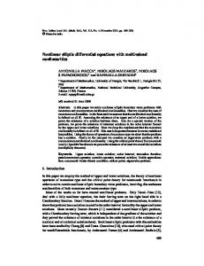
Partial differential systems with nonlocal nonlinearities

Partial differential systems with nonlocal nonlinearities

Suggest Documents

Homogenization of Periodic Linear Nonlocal Partial Differential

Nonlinear elliptic differential equations with multivalued nonlinearities

Partial Differential Equations with Maple

Damage Detection in Dynamic Systems with Nonlinearities

Nonlinear perturbations of systems of partial differential equations with

Multidimensional partial differential equation systems - UBC Math

Multidimensional partial differential equation systems - UBC Math

Nonlinear Partial Differential Equations, Dynamical Systems and ...

Coupled Systems of Differential Algebraic and Partial Differential ...

Coupled Systems of Differential Algebraic and Partial Differential

A class of nonlocal indefinite differential systems - Boundary Value ...

Gap solitons under competing local and nonlocal nonlinearities

PARTIAL DIFFERENTIAL EQUATIONS WITH ROBIN ... - public.asu.edu

Note on Partial Differential Equations with Non

The solutions of partial differential equations with

On the Partial Differential Equations with Non

Partial Differential Equations

Partial Differential Equations

Partial differential equations [PDF]

Partial Differential Equations

Partial Differential Equations

Stochastic Partial Differential Equations

Partial Differential Equations - METU

SOLVING PARTIAL INTEGRO-DIFFERENTIAL