Mokhtaria Mesri 1*, Khaled Tahkoubit2, Hocine Merrah1 Adda Ali-pacha2
J. Electrical Systems 13-1 (2017): 169-182 Regular Paper Partial Transition Sequence Algorithms for Reducing Peak to Average Power Ratio in the Next Generation Wireless Communications Systems
JES Journal of Electrical Systems
The unprecedented scientific and technical advancements along with the ever-growing needs of humanity resulted in a revolution in the field of communication. Hence, single carrier waves are being replaced by multi-carrier systems like Orthogonal Frequency Division Multiplexing (OFDM) and Generalized Frequency Division Multiplexing (GFDM) which are nowadays commonly implemented. In the OFDM system, orthogonally placed subcarriers are used to carry the data from the transmitter to the receiver end. The presence of guard band in these systems helps in dealing with the problem of intersymbol interference (ISI) and noise is minimized by the larger number of subcarriers. However, the large Peak to Average Power Ratio (PAPR) of these signals has undesirable effects on the system. PAPR itself can cause interference and degradation of Bit Error Rate (BER). To reduce High Peak to Average Power Ratio and Bit Error Rate problems, more techniques are used. Furthermore, each technique has its own disadvantages, such as complexity in-band distortion and out-of-band radiation into OFDM and GFDM signals. In this paper, the emphasis will be put on the GFDM systems as well as on the methods that are meant to reduce the PAPR problem and improve efficiency. Keywords: GFDM, ISI, MIMO, OFDM, PAPR, PTS Article history: Received 20 December 2016, Accepted 12 February 2017
1. Introduction The successful deployment of killer applications in wireless communication technology led to its rapid development in the past 20 years with a major impact on modern life and on the way societies operate in politics, economy, education, entertainment, logistics & travel, and industry. The evolution of wireless communication systems technologies can be discretely grouped into various generations based on the level of maturity of the underlying technology. The classification into generations is not standardized on any given metrics or parameters and as such does not represent a clear-cut demarcation. However, it represents a perspective which is commonly agreed upon, both by industry and academia, and subsequently conceived to be an unwritten standard. The so called Long Term Evolution is a wireless communication standard commonly known as 4G LTE. It is developed by third Generation Partnership Project (3GPP) and based on packet switched network and Internet Protocol (IP) [1]. Currently, OFDM has been chosen for Digital Audio Broadcasting (DAB), Digital Video Broadcasting (DVB) and Wireless Local Area Networks (WLAN) technology based on the standards IEEE 802.11 [2]. OFDM applications have been extended from high frequency radio communication to telephone networks. In OFDM, the subcarriers are chosen to be orthogonal to each other. This is done by breaking the wideband transmit signal into many narrowband subchannels. *
Corresponding author: M. Mesri, Electronics Department, University Amar Telidji, BP 37G, Laghouat 03000, Algeria, Email :
[email protected] 1 Electronics Department, University Amar Telidji, BP 37G, Laghouat 03000, Algeria 2 Laboratory of coding, University of science and technology of Oran, 31000 Algeria
Copyright © JES 2017 on-line : journal/esrgroups.org/jes
J. Electrical Systems 13-1 (2017): 169-182
The orthogonality of the carriers means that each carrier has an integer number of cycles over a symbol period. As a result, the spectrum of each carrier has a null at the center frequency of each of the other carriers in the system. This results in no interference between the carriers [3]. The generalized frequency-division multiplexing (GFDM) is a recently proposed multicarrier modulation method which employs cyclic-prefixed (CP) block signal transmission as the orthogonal frequency-division multiplexing (OFDM), but it is endowed with a more flexible time-frequency signal structure [4, 5]. It is, however, observed that, under some signal configurations, the transmitter filter bank does not have full rank, adversely affecting the transmission capacity [5, 6]. In particular, this phenomenon does not happens unless there is an even number of sub-symbols in a GFDM symbol, an even number of subcarriers and a certain symmetry in the prototype filter response. Apart from singularity, it is also known that a typical GFDM filter bank may have unequal magnitude gains in different vector-space dimensions [6]. High PAPR causes severe degradation of Bit Error Rate (BER) performance. In addition, in-band and out-of-band distortion occurs in the non-linear amplifier and leads to power inefficiency in the Radio Frequency (RF) section of the transmitter. There are different techniques for PAPR reduction [7, 8] including Selective Mapping (SLM) [9], Tone Reservation (TR) [10], Clipping and Filtering [11] and Partial Transmit Sequence (PTS) [12, 13]. PTS is regarded as one of the best techniques to reduce the PAPR in GFDM systems. 2. GFDM Systems Generalized Frequency Division Multiplexing (GFDM) is a candidate waveform that has been investigated as a component in the physical layer (PHY) of future wireless communication systems. Particularly, GFDM can use Time-Frequency Localization (TFL) of the transmit signal to address spectral agility and aggregation of carriers with an adaptation of the prototype filter and resource grid. However, inherent self-interference between subcarriers of GFDM hinders the application of standard spatial multiplexing (SM) detection algorithms. A data source provides the binary data vector b , which is encoded to obtain bc . A mapper, e.g. QAM Modulation, maps the encoded bits to symbols from a 2μ-valued complex constellation where μ is the modulation order. The resulting vector d denotes a data block that contains N elements, which can be decomposed into K subcarriers with M
(
T sub-symbols, each according to d c = d 0T , … , d M −1
)
T
and d m = (d 0,m , … , d k −1,m )T . The
total number of symbols follows as N = KM . The individual elements dk,m correspond to the data transmitted on the kth subcarrier and in the mth subsymbol of the block. The details of the GFDM modulator are shown in equation (1). Each dk,m is transmitted with the corresponding pulse shape: k g k , m [n] = g [(n − mK ) mod N ]. exp − j 2π K With n denoting the sampling index, each
(1) n g k ,m [n] is a time and frequency shifted version
of a prototype filter g [n] , where the module operation makes g k ,m [n] a circularly shifted version of g k ,0 [n] and the complex exponential performs the shifting operation in
170
M Mesri et al: Partial Transition Sequence Algorithms for Reducing Peak to Average... Average...
frequency. The transmit samples x = (x[n])T are obtained by superposition of all transmit symbols:
x[n] =
∑ ∑ K −1
M −1
k =0
m=0
g k , m [n]d k ,m , n = 0, … , N − 1
(2)
Collecting the filter samples in a vector g k ,m = (g k ,m [n])T allows formulating Equation (2) as
x = Ad Where A is a KM × KM transmitter matrix with a structure according to:
(3)
A = (g 0,0 ,…, g k −1,0 , g 0,1 ,…, g k −1,m−1 )
(4)
As one can see, g1,0 = [A]n, 2 and g 0,1 = [A]n,K +1 are circularly frequency and timeshifted versions of, g 0,0 = [A]n,1 . At this point, x contains the transmit samples that correspond to the GFDM data block d . Lastly, on the transmitter side, a cyclic prefix of N CP samples is added to produce x . 2.1. Peak to Average Power Ratio (PAPR)
Due to the large number of sub-carriers in typical Multicarrier Modulation (MCM) systems, the amplitude of the transmitted signal has a large dynamic range, leading to inband distortion and out-of-band radiation when the signal passes through the nonlinear region of the power amplifier. Peak Power is defined as: j 2πki k −1 Max x(t ) ∗ x (t ) = Max ak e T 0 Average power is as follows:
[
]
∗
∑
∑
k −1 ∗ ak e 0
− j 2πki T
j 2πki − j 2πki k −1 k −1 ∗ E x(t )x∗ (t ) = E ak e T ak e T 0 0 So, mathematically PAPR is given by,
[
] ∑
[
∑
] [
]
PAPR = Max x(t )x ∗ (t ) E x(t )x ∗ (t )
(5)
(6)
(7)
The Complementary Cumulative Distribution Functions CCDF formula that approximates the PAPR of a multicarrier signal with Nyquist sampling rate is derived from the central limit theorem [6] and is given by: − x2 2
CCDF ( PAPR0 ) = 1 − (1 − e 2σ ) N
(8)
2.2. Solid-State Power Amplifier (SSPA)
171
J. Electrical Systems 13-1 (2017): 169-182
The SSPA [14] shows non-linear characteristics as it causes distortion of the signals, particularly high PAPR values. Consequently, the BER performance of the system is decreased. The Rapp model of Solid-State Power Amplifier (SSPA) is defined by following Amplitude-to-Amplitude Modulation (AM/AM) and Amplitude-to-Phase Modulation (AM/PM) characteristics:
Vin
Vout =
(1 + ( Vin / U sat )
(9)
1 2p 2p
)
Where p is the smoothness factor and U sat is the output saturation level. 2.3. The Partial Transmit Sequence (PTS) Technique PTS scheme [12] is a common method to reduce PAPR of an OFDM signal. Its basic principle can be described as follows: Let X be an input symbol sequence as presented in Equation (10):
X = [X 0 , X1 ,……, X N ]
(10)
This sequence is then partitioned {X v , v = 1,2,…,V } as in Equation (11):
X=
∑
V v =1
into
V “disjoint” symbol
subsequences
(11)
Xv
{
}
It introduces rotating vector: av = e jθv , v = 1,2,…,V ;θ v ∈ [0,2π ] which is known as Side Information (SI), where each signal subsequence Xv is multiplied by a unit magnitude constant av, to generate what is given by Equation (12):
Y=
∑
V
(12)
a X v =1 v v
One can get time-domain signal through IFFT, as expressed in Equation (13):
y = IFFT (Y ) =
∑
V
(13)
a X v =1 v v
PAPR value is then compared by selecting different phase factors so as to yield the phase factor vector for OFDM signals with the minimum PAPR. The corresponding objective function can be written as in Equation (14):
[a1 , a2 ,……, av ] = arg min(max ∑v=1 av X v V
2
)
(14)
Where ‘arg min’ stands for the decision condition at the minimum value of the function. So PAPR performance of the GFDM system is improved through finding the best phase factor {av , v=1,2,…..,V } at the cost of V −1 times IFFT. Figure 1 shows a typical GFDM system with traditional PTS.
172
M Mesri et al: Partial Transition Sequence Algorithms for Reducing Peak to Average... Average...
Figure 1: PTS method block. 3. Different PTS techniques
In the PAPR reduction process, PTS does not deteriorate the orthogonality of subcarriers, but it needs lots of IFFTs and requires an exhaustive search over all combinations of allowed weighting coefficients, which brings a much higher computational load. Several solutions have been proposed recently [11] to tackle this issue. Modified PTS technique is an effective way to cut down the computational complexity; however, the performance of PAPR is still a limitation, compared with the ordinary PTS technique. Modified PTS with the interleaving scheme is suggested by using interleaved sub-block partition and pulse shape technique to avoid multiple IFFT in PAPR reduction. Although this method reduces computational complexity, it does not improve well the PAPR performance. In the present work, we will shed light on two types of methods: Probabilities-PTS, such as Optimal-PTS, Random Search PTS, and others, and Artificial PTS, such as ABC-PTS and BFO-PTS which are based on artificial behavior. 3.1. Probabilities Algorithms
a. Optimal-PTS
The Optimal PTS (O-PTS) [15] is a promising technique that can reduce the PAPR, while its complexity increases rapidly as the number of sub-blocks increases. Let X denote a random input signal in frequency domain with length N. X is partitioned into V disjoint sub-blocks X=[X0, X1, X2…….XN-1]T which are then combined to minimize the PAPR in time domain. The sub-block partition is based on interleaving in which the computational complexity is less compared to adjacent and Pseudo-random; however, it has the worst PAPR performance among them. By applying the phase rotation factor bv= ejᴓv, v= 1,2,3,…….V to the IFFT of the vth subblock Xv, the time domain signal after combining is given by:
x′(b) =
∑
V
b x v =1 v v
(15)
173
J. Electrical Systems 13-1 (2017): 169-182
Where x′(b ) = [x0′ (b ), x1′ (b ),…, x NL−1 (b )]T and L is the over sampling factor. The objective is to find the optimum signal x'(b) with lowest PAPR. Both b and x can be shown in matrix form as follows:
b1 ⋯ b1 b = ⋮ ⋮ ⋮ bv ⋯ bv N ∗V
(16)
b1,0 ⋯ b1, NL−1 b= ⋮ ⋮ ⋮ bv,0 ⋯ bv , NL−1
(17) NL −1∗V
It should be noted that all elements of each row of matrix b are of same values, and this is in accordance with O-PTS method. In order to have exact PAPR calculation, at least 4 times oversampling is necessary. As oversampling of x adds zeros to vector, the number of phase sequences to multiply to matrix x will remain same. Now, the process is performed by choosing optimization parameter b' according to the following condition: V (18) b′ = arg min max bv xv 0≤ K ≤ NL−1 v−1 Once the optimum b' is found, the optimum signal is transmitted to the next block. Finding optimum b', requires performing an exhaustive search for (V-1) phase factors since one phase factor can remain fixed, b1=1. Hence WV-1 iterations should be performed to find optimum phase factor, where W is the number of allowed phase factors.
∑
b. Random Search (RS-PTS) Random search algorithms [17] are useful for many global optimization problems with continuous and/or discrete variables. Typically random search algorithms sacrifice a guarantee of optimality for finding a good solution quickly with convergence results in probability. Random search algorithms include mainly: simulated annealing, genetic algorithms, evolutionary programming, particle swarm optimization and colony optimization. A random search algorithm refers to an algorithm that uses some kind of randomness or probability (typically in the form of a pseudo-random number generator). This method may be called a Monte Carlo method or a stochastic algorithm as referred to as in the literature. The term metaheuristic is also commonly associated with random search algorithms. The problem of designing algorithms that obtain global optimal solutions is very difficult when there is no overriding structure that indicates whether a local solution is indeed a global one. c. I-PTS In this section, I-PTS algorithm for PAPR reduction is considered [16], in that it presents a problem of traversing the binary tree. The solution of I-PTS is always updated for improvements purposes and is quickly trapped in a local optimum. Therefore, instead of using the linear search of I-PTS, the Metropolis criterion is applied to decide whether the current phase factor
174
M Mesri et al: Partial Transition Sequence Algorithms for Reducing Peak to Average... Average...
b = {bm ; m = 1,2,…, M } is accepted or rejected. This can be described within the following steps: 1 -Suppose that b' is the phase factor obtained from the previous search and ∆E = PAPR(b)PAPR(b'). 2-if ∆E ≤ 0, accept the move and keep the current b. − ∆E probability e TK
, where Tk = α ⋅ Tk −1 ;α ∈ [0.8,1] . 3-if ∆E > 0, accept the move with 4- The phase factor which does not show the minimum PAPR may be chosen; thus, the local optimum convergence can be avoided and the PAPR performance is improved consequently. Moreover, due to the linear search of I-PTS, a different selection of initial phase factor may show diverse PAPR performance. Another iteration PTS is to eliminate the effect of initial phase factor. The phase factor that is achieved by the previous iteration is set as the initial phase factor of the current search; as a consequence, the search becomes closer to the optimal phase factor. The optimum phase factor with minimum PAPR is then obtained after U times. It is crucial to note that more cyclic time provides a better performance, but with a higher complexity. Therefore, an appropriate U should be chosen to obtain the good compromise between PAPR performance and complexity. The PTS algorithm should perform an exhaustive search for M phase factors; consequently, D = WM sets of phase factors are searched to find the optimum set of phase factors. The search complexity increases exponentially with the number of sub-blocks M. IPTS needs M sets of search to find the sub-optimum phase factors with much PAPR performance decline. 3.2. Artificial Algorithms
a. Artificial Bee Colony (ABC-PTS) This algorithm was recently proposed by Karaboga [15]. In the ABC algorithm, employed bees, onlooker bees, and scout bees are tasked with finding optimum food sources, and first, the food source positions are generated randomly. In the PAPR reduction problem, a food source position is equivalent to phase vector bi = [bi1, bi2, bi(V−1)] where i = 1,…., SN, and SN denotes the population size, which is composed of the employed bees or the onlooker bees. The employed bees look for a new food source within the neighborhood of the previous source. If the nectar amount of the new source is higher than the previous one, the new source is memorized as a possible optimum solution. In the ABC-PTS, the new phase vector (the new food source) is expressed by (19) bi′ = bi + ϕ i (bi − bK ) Where bk is a solution within the neighborhood of bi , and ϕ i is a random number in the range of [−1, 1] . The nectar amount of the food source determines the quality or fitness of the solution that is expressed as:
1 iff (bi ) ≥ 0 fit (bi ) = 1 + f (bi ) 1 + abs( f (b ))iff (b ) ≺ 0 i i
(20)
175
J. Electrical Systems 13-1 (2017): 169-182
Where f (bi) represents the PAPR value of the signal and is desired to be at a minimum. The probability of an onlooker bee selecting a food source is calculated as:
pi =
fit (bi )
∑
SN
i =1
(21)
fit (bi )
After an onlooker bee reaches a food source, it looks for a new source within the neighborhood of the previous one and memorizes the food sources according to their fitness. After the employed bees and onlooker bees complete their searches, if the fitness values of the food sources do not improve with a number of iterations that is called the “limit” value, employed bees become the scout bees. The scout bees look for new food sources randomly by: (22) bi = min (bi ) + rand (0,1) ∗ (max (bi ) − min (bi )) Where min (bi) and max (bi) are the lower and upper bounds of the phase vector. The above steps are repeated within a cycle, called the maximum number of cycles (MCN). In a cycle, possible SN solutions are produced. In the ABC-PTS algorithm, MCN ∗ SN possible solutions are produced to find the optimum phase vector. b. Bacterial Foraging Optimization (BFO-PTS)
Figure 2: Flowchart of BFO E. coli recently introduced the Bacterial Foraging Optimization algorithm (BFO) [18] for numerical optimization problems. The Flowchart of BFO is shown in Figure 2.
176
M Mesri et al: Partial Transition Sequence Algorithms for Reducing Peak to Average... Average...
4. Computational Complexity When the number of subcarriers is N = K ⋅ M = 2 n , the numbers of complex multiplication n mul and complex addition n add of the conventional PTS-GFDM scheme
are given by n mul = 2 n −1 ⋅ n ⋅ V and n add = 2 n ⋅ n ⋅ V where V is the number of sub-blocks. Thus, the computational complexity reduction ratio (CCRR) of the new PTS GFDM scheme over the conventional PTS GFDM scheme is defined as:
complexity⋅ of ⋅ new ⋅ PTS × 100 CCRR = 1 − complexity ⋅ of ⋅ conventional ⋅ PTS
Table 1: Complexity analysis of the PTS schemes Method
Complexity of new PTS
Normalized computational time
Complexity of conventional PTS (O-PTS)
RS-PTS
4096
12.79
32 768
I-PTS
30
0.09
32 768
ABC-PTS
16
0.10
32 768
ABC-PTS
64
0.28
32 768
ABC-PTS
1024
3.68
32 768
BFO-PTS
320
1.2
32 768
BFO-PTS
900
2.2
32 768
The CCRRs for the O-PTS scheme compared to the RS-PTS, I-PTS, ABC-PTS and BFO-PTS for different values of N and V are presented in Table 2. It is obvious from Table 2 that the I-PTS scheme has a lower computational complexity than both the ABC-PTS and BFO-PTS schemes, especially when increasing the number of sub-blocks V. Table 2: Computational Complexity Reduction Ratio CCRR % N=256
Method
N=512
N=1024
v=
4
8
16
4
8
16
4
8
16
RS-PTS
11.8
17.5
32.2
22.1
25.7
48.1
41.1
50.4
55.1
I-PTS
11.2
17.1
31.8
21.2
24.8
47.2
40.7
49.9
52.2
ABC-PTS
13.7
20.3
38.2
29.1
34.7
53.1
48.2
54.3
59.4
BFO-PTS
13.4
20.1
37.7
28.7
33.1
51.2
46.9
52.1
58.2
177
J. Electrical Systems 13-1 (2017): 169-182
5. Simulation results
The Performance of GFDM was tested through computer simulation by setting the parameters as shown in Table 1. Table 3: GFDM parameters Parameter
Notation
Value
Modulation
-
QAM 16
Samples per symbol
N
256
No. of active subcarriers
K
64
Block size(symbols)
M
256
Sampling frequency(MHz)
Fs
2
Symbol duration(μs)
Ts
60
Block duration (μs)
Tb
60
Channel model
-
AWGN, Rayleigh
5.1. PAPR Reduction
Figure 3: Comparison between probabilities algorithms Figure 3 reveals that the best algorithm to reduce PAPR is O-PTS, but the problem of complexity and search number still remains. Random search algorithm also provides good results with only 256 search. 178
M Mesri et al: Partial Transition Sequence Algorithms for Reducing Peak to Average... Average...
Figure 4: Comparison of PAPR performance (Nc =2,4,6 ) Figure 4 shows the PAPR reduction performance with a different number of chemotactic loop Nc. As Nc increases, the PAPR performance of BFA-PTS has small improvement while the computational complexity becomes high accordingly. Therefore, an appropriate iteration number Nc=4 is the best choice to achieve the excellent PAPR reduction performance with very low complexity. Similarly, the variable PAPR performance caused by different swim length Ns, and the perfect swim length is chosen as Ns= 4. 5.2. BER Performance
Figure 5: The Performance of GFDM without HPA in AWGN channel. 179
J. Electrical Systems 13-1 (2017): 169-182
-1
10
16-QAM-GFDM without HPA 64-QAM-GFDM without HPA 256-QAM-GFDM without HPA) -2
10
-3
BER
10
-4
10
-5
10
0
5
10
15
20 SNR(dB)
25
30
35
40
Figure 6: The Performance of GFDM without HPA in Rayleigh Fading channel. Figures 5 and 6 represent the performance of GFDM system using different modulations: 16-QAM, 64-QAM and 256-QAM in a Gaussian channel and Rayleigh Fading channel without channel coding. We note that the results of the 16-QAM modulation are better than those obtained by the modulation 64QAM and 256-QAM.We can conclude that performance of the system decreases when the number of constellations increases.
Figure 7: Performance of GFDM in the presence of SSPA in AWGN channel
180
M Mesri et al: Partial Transition Sequence Algorithms for Reducing Peak to Average... Average...
Figure 8: Performance of GFDM with HPA in Rayleigh Fading channel. Figures 7 and 8 represent the performance of GFDM system in the presence of SSPA model with a Gaussian channel (AWGN) and a multipath channel (Rayleigh Fading channel).We can note that the system is affected by the use of high power amplifier while the aim of this work is to reduce PAPR to improve the performance of the system. Simulation results show that the performance of the system decreases when the value of IBO decreases, which means the level of the saturation of the amplifier diminish. 6. Conclusion
In this paper, almost all Partial Transmit Sequence (PTS) techniques for PAPR reduction in GFDM system are undertaken. Simulations results show that Optimum-PTS technique is the most preeminent method for PAPR reduction, though its drawbacks are optimization of Phase factor and complexity. Random-Search PTS technique is an effective method to reduce the PAPR. It makes use of random optimization and sub-block circular permutation which reduce the computational complexity and equivalently improve the performance for PAPR reduction. We believe that this paper may provide an important contribution to the research community by documenting the various PTS techniques and their applications in the GFDM system and helping readers interested in PAPR reduction and BER issues. This is the first paper involved in Peak to Average Power Ratio in GFDM system. References Raj Jain “Long Term Evolution (LTE) & Ultra-Mobile Broadband (UMB) Technologies for Broadband Wireless Access” Wireless and Mobile Networking (Spring 2008), Last Modified: April, 2008 . [1] J.Armstrong,“OFDM for optical communications”, Journal of Light wave Technology, vol.27,no.3, pp.189–204, February 2009. [2] P.Mukunthan, K.Rajalakshmi, K.Tamilselvi, N.Vinothini “Papr Reduction Based on PTS Combined Interleaving and Analysis of BER using Hadamard Code in OFDM
181
J. Electrical Systems 13-1 (2017): 169-182
Systems“ International Conference on Communication and Signal Processing, April 68, 2016, India . [3] G. Fettweis, M. Krondorf, and S. Bittner, “GFDM Generalized Frequency Division Multiplexing,” in Proc. IEEE 69th Veh. Technol. Conf., Apr. 2009, pp. 1–4. [4] Nicola Michailow, Maximilian Matthé, Ivan Simões Gaspar, Anima Navarro Caldevilla,Luciano Leonel Mendes, Andreas Festag, Senior Member, IEEE, and Gerhard Fettweis, Fellow, IEEE," Generalized Frequency Division Multiplexing for 5th Generation Cellular Networks", IEEE TRANSACTIONS ON COMMUNICATIONS, VOL. 62, NO. 9, SEPTEMBER 2014. [5] M. Matthe, L. L. Mendes, and G. Fettweis, “Generalized frequency division multiplexing in a Gabor transform setting,” IEEE Commun. Lett., vol. 18, no. 8, pp. 1379–1382, Aug. 2014. [6] Goldsmith Andreas “Wireless Communication” Cambridge University Press 2005 pp.299-318, 367- 370, 417-439. [7] R. Prasad, OFDM for Wireless Communications System .Artech House, Inc., 2004 pp. 33-51, 119- 153. [8] Xiao, Y., Chen, M., Li, F., Tang, J., Liu, Y., & Chen, L. (2015). PAPR reduction based on chaos combined with SLM technique in optical OFDM IM/DD system. Optical Fiber Technology, 21, 81-86. [9] Xia, J., Li, Y., Zhang, Z., Wang, M., Yu, W., & Wang, S. (2013, April). A suboptimal TR algorithm with fixed phase rotation for PAPR reduction in MC-CDMA system. In Informa-tion and Communications Technologies (IETICT 2013), IET International Conference on (pp. 415-420). IET. [10] Ragusa, S., Palicot, J., Louët, Y., &Lereau, C. (2006). Invertible clipping for increasing the power efficiency of OFDM amplification.In ICT 2006. [11] Sarala, B., Venkateswarulu, D. S., &Bhandari, B. N. (2012). Overview of McCdma PAPR Reduction Techniques.arXiv preprint arXiv:1204.3874. [12] Baig, I., Ayaz, M., &Jeoti, V. (2013). A SLM based localized SC-FDMA uplink system with reduced PAPR for LTE-A. Journal of King Saud University-Engineering Sciences, 25(2), 119-123. [13] C. Rapp, “Effects of the HPA-nonlinearity on a 4-DPSK/OFDM signal for a digital sound broadcasting system,” in Proc. ECSC’91, Luettich, Oct. 1991. [14] Blum, C., and Roli, A., (2003) “Metaheuristics in Combinatorial Optimization: Overview and Conceptual Comparison,” ACM Computing Surveys, 35(3), 268-308. [15] Leman Dewangan, Mangal Singh, NeelamDewangan, "A Survey of PAPR Reduction Techniques in LTE-OFDM System" , International Journal of Recent Technology and Engineering (IJRTE) ISSN: 2277-3878, Volume-1, Issue-5, November 2012 [16] N.TASPINAR, D.KARABOGA, M.YILDIRIM, B.AKAY "PAPR reduction using artificial bee colony algorithm in OFDM systems", Turk J ElecEng& Comp Sci, Vol.19, No.1, 2011. [17] R. Manjith M. Suganthi" Peak to Average Power Ratio Reduction using a Hybrid of Bacterial Foraging and Modified Cuckoo Search Algorithm in MIMO-OFDM System", Research Journal of Applied Sciences, Engineering and Technology (2014 / 06 / 05) P4423 - 4433 . [18] Er. Ankita, Anand Nayyar "Review of various PTS (Partial Transmit Sequence) techniques of PAPR (Peak to Average Power Ratio) reduction in MIMO-OFDM ", International Journal of Innovative Technology and Exploring Engineering (IJITEE) ISSN: 2278-3075, Volume-2, Issue-4, March 2013.
;
,
182
;