Partially Observable Markov Decision Processes with Continuous Ob ...

6th SIGdial Workshop on Discourse and Dialogue Lisbon, Portugal September 2-3, 2005

ISCA Archive

http://www.isca-speech.org/archive

Partially Observable Markov Decision Processes with Continuous Observations for Dialogue Management Jason D. Williams Cambridge University Engineering Department Trumpington Street Cambridge CB2 1PZ UK

Pascal Poupart School of Computer Science University of Waterloo 200 University Avenue West Waterloo, ON, N2L 3G1 Canada

Steve Young Cambridge University Engineering Department Trumpington Street Cambridge CB2 1PZ UK

[email protected]

[email protected]

[email protected]

Abstract This work shows how a dialogue model can be represented as a Partially Observable Markov Decision Process (POMDP) with observations composed of a discrete and continuous component. The continuous component enables the model to directly incorporate a confidence score for automated planning. Using a testbed simulated dialogue management problem, we show how recent optimization techniques are able to find a policy for this continuous POMDP which outperforms a traditional MDP approach. Further, we present a method for automatically improving handcrafted dialogue managers by incorporating POMDP belief state monitoring, including confidence score information. Experiments on the testbed system show significant improvements for several example handcrafted dialogue managers across a range of operating conditions.

1

Introduction

Dialogue management is a difficult problem for several reasons. First, speech recognition errors are common, corrupting the evidence available to the machine about a user’s intentions. Second, a user may change their intentions at any point – as a result, the machine must decide whether conflicting evidence has been introduced by a speech recognition error, or by a new user intention. Finally, the machine must make trade-offs between the “cost” of gathering additional information (increasing its certainty of the user’s goal, but prolonging the conversation) and the “cost” of committing to an incorrect user goal. That is, the system must perform planning to decide what sequence of actions to take to best achieve the user’s goal despite having imperfect

information about that goal. For all of these reasons, dialogue management can be cast as planning under uncertainty. In this context, making use of any “clues” about speech recognition accuracy ought to improve the performance of a dialogue manager. In this paper, we are interested in one such clue: confidence score. A confidence score is a real-valued metric intended to provide a clue about the reliability of a recognition hypothesis. This paper addresses how confidence score can be incorporated into the dialog management problem when viewed as planning under uncertainty. Planning under uncertainty can be approached as a (fully observable) Markov decision processes (MDP) or a partially observable Markov decision process (POMDP), and both of these techniques have been applied to dialog management. The application of MDPs was first explored by Levin and Pieraccini (1997). Levin et al. (2000) provide a formal treatment of how a MDP may be applied to dialogue management, and Singh et al. (2002) show application to real systems. However, MDPs assume the current state of the environment (i.e., the conversation) is known exactly, and thus they do not naturally capture the uncertainty introduced by the speech recognition channel. Partially observable MDPs (POMDPs) extend MDPs by providing a principled account of noisy observations. Roy et al. (2000) compare an MDP and a POMDP version of the same spoken dialogue system, and find that the POMDP version gains more reward per unit time than the MDP version. Further, the authors show a trend that as speech recognition accuracy degrades, the margin by which the POMDP outperforms the MDP increases. Zhang et al. (2001) extend this work in several ways. First, the authors add “hidden” system states to account for various types of dialogue trouble, such as different sources of speech recognition errors. Second, the authors use Bayesian networks to combine observations from a variety of sources (including confidence score). The authors again show that the

POMDP-based methods outperform MDP-based methods. In all of these proposals, the authors have incorporated confidence score by dividing the confidence score metric into regions, often called “confidence buckets.” For example, in the MDP literature, Singh et al. (2002) tracks the confidence bucket for each field as “high, medium, or low” confidence. The authors do not address how to determine an “optimal” number of confidence buckets, nor how to determine the “optimal” thresholds of the confidence score metric that divide each bucket. In the POMDP literature, Zhang et al. (2001) use Bayesian networks to combine information from many continuous and discrete sources, including confidence score, to compute probabilities for two metrics called “Channel Status” and “Signal Status”. Thresholds are then applied to these probabilities to form discrete, binary observations for the POMDP. However, it is not clear how to set these thresholds to maximize POMDP return. Looking outside the (PO)MDP framework, Paek and Horvitz (2003) suggest using an influence diagram to model user and dialogue state, and selecting actions based on “Maximum Expected [immediate] Utility.” This proposal can be viewed as a POMDP with continuous observations that greedily selects actions – i.e., which selects actions based only on immediate reward.1 By choosing appropriate utilities, the authors show how local grounding actions can be automatically selected in a principled manner. In this work, we are interested in POMDPs as they enable planning over any horizon. This paper makes two contributions. First, we show how a confidence score can be accounted for exactly in a POMDP-based dialogue manager by treating confidence score as a continuous observation. Using a testbed simulated dialog management problem, we show that recent optimization techniques produce policies which outperform traditional MDP-based approaches across a range of operating conditions. Second, we show how a hand-crafted dialogue manager can be improved automatically by treating it as a POMDP policy. We then show how a confidence score metric can be easily included in this improvement process. We illustrate the method by presenting three handcrafted controllers for the testbed dialog manager, and show that our technique improves the performance of each controller significantly across a variety of operating conditions. The paper is organised as follows. Section 2 briefly reviews background on POMDPs. Section 3 presents our method for incorporating confidence score into a POMDP-based dialogue manager. Section 4 outlines 1

We can express this formally as a POMDP with discount λ = 0 . See section 2 for background on POMDPs.

our testbed dialogue management simulation. Section 5 compares policies produced by our method vs. an MDP baseline on the testbed problem. Section 6 shows how a handcrafted policy can be improved using confidence score, and provides an illustration, again using the testbed problem. Section 7 concludes.

2

Overview of POMDPs

Formally, a POMDP is defined as a tuple {S, Am, T, R, O, Z}, where S is a set of states, Am is a set of actions that an agent may take,2 T defines a transition probability p ( s ′ | s, a m ) , R defines the expected (immediate, real-valued) reward r ( s, a m ) , O is a set of observations, and Z defines an observation probability, p(o′ | s′, am ) . In this paper, we will consider POMDPs with discrete S and continuous O. The POMDP operates as follows. At each time-step, the machine is in some unobserved state s . The machine selects an action am , receives a reward r , and transitions to (unobserved) state s ′ , where s ′ depends only on s and am . The machine receives an observation o ′ which is dependant on s ′ and am . Although the observation gives the system some evidence about the current state s , s is not known exactly, so we maintain a distribution over states called a “belief state,” b. We write b(s ) to indicate the probability of being in a particular state s. At each timestep, we update b as follows: b′( s′) = p( s′ | o′, am , b)

b′( s′) =

(1)

p (o′ | s′, am )∑ p ( s′ | am , s )b( s ) s∈S

p ( o′ | a m , b )

.

(2)

The numerator consists of the observation function, transition matrix, and current belief state. The denominator is independent of s′ , and can be regarded as a normalisation factor; hence: b′( s′) = k ⋅ p (o′ | s′, am )

∑ p ( s′ | a

m

, s )b( s ) .

(3)

s∈S

We refer to maintaining the value of b at each time-step as “belief monitoring.” The immediate reward is computed as the expected reward over belief states:

2

In the literature, the system action set is often written as an un-subscripted A. In this work, we will model both machine and user actions, and have chosen to write the machine action set as Am for clarity.

ρ (b, am ) = ∑ b( s)r ( s, am ) ,

(4)

s∈S

A policy specifies an action to take given a belief state.3 The goal of the machine is to find a policy which maximises the cumulative, infinite-horizon, discounted reward called the return: ∞

∑ λ ρ (b , a t =0

t

t

∞

mt

) = ∑ λt ∑ bt ( s ) r ( s, am t ) t =0

(5)

s∈S

where bt indicates the distribution over all states at time t, bt (s ) indicates the probability of being in state s at timestep t, and λ is a geometric discount factor, 0 ≤ λ ≤ 1. Because belief space is real-valued, an optimal infinite-horizon policy may consist of an arbitrary partitioning of S-dimensional space in which each partition maps to an action. In fact, the size of the policy space grows exponentially with the size of the (discrete) observation set and doubly exponentially with the distance (in timesteps) from the horizon (Kaelbling et al., 1998). A continuous observation space compounds this further. Nevertheless, real-world problems often possess small policies of high quality. In this work, we make use of two recent approximate methods. The first, Perseus (Spaan and Vlassis, 2004), operates on problems with discrete observation sets and is capable of rapidly finding good yet compact policies (when they exist). Perseus heuristically selects a small set of representative belief points, and then iteratively applies value updates to just those points, instead of all of belief space, achieving a significant speed-up. Perseus has been tested on a range of problems, and found to outperform a variety of other methods, including grid-based methods (Spaan and Vlassis, 2004). The second method is an extension to Perseus proposed by Hoey and Poupart (2005) which operates on POMDPs with continuous or very large discrete observation sets. This method exploits the fact that different observations may lead to identical courses of action to discretize continuous observations without any loss of information. In the context of dialogue management with a continuous confidence score, it implicitly and adaptively finds optimal lossless buckets of confidence that are equivalent to using the original continuous confidence score.4

3 We will assume the planning horizon for a policy is infinite unless otherwise stated. 4 The actual implementation used in this paper approximates some integrals by Monte Carlo sampling, which means that the confidence buckets are not exactly lossless.

3

Method

This section presents our method for incorporating confidence score into the POMDP as a continuous observation. First, we decompose the observation o into a discrete component h and a continuous component c. The discrete component represents the speech recogntion hypothesis, and the continuous component represents the confidence score. 5 The observation function then becomes p(h′, c′ | s′, am ) . Next, we will assume that am does not affect recognition directly – i.e., h′ and c′ are conditionally dependent on only s′ . Thus the observation function becomes: p(h′, c′ | s′, am ) = p(h′, c′ | s′) = p(h, c | s ). .

(6)

This distribution expresses the probability density of observing hypothesis h with confidence score c in state s. In the POMDP model, s includes unobserved elements of the current state, such as the user’s true action. As such, the observation function can be viewed as a model of the errors introduced by the speech recognition channel. In practice this distribution will be impossible to estimate directly from data, so we make several assumptions. First, we assume that the state s can be factored in order to condition {h,c} on fewer elements. For example, the observation will depend directly on the user’s (actual, unobserved) action/utterance au and possibly the current grammar g selected by the machine. However, the observation will not directly depend on the (unobserved) user’s goal. Second, we can decompose the distribution by assuming that confidence scores are drawn from just two distributions – one for “correct” recognitions and another for “incorrect” recognitions. Combining both of these assumptions, we write:  pcorrect (c) ⋅ p(h | au , g ) if h = au p(h, c | s ) ≈   pincorrect (c) ⋅ p(h | au , g ) if h ≠ au

(7)

where: •

p(h | au , g ) expresses the confusion matrix – i.e., probability of observing hypothesis h given that the user took action a u , and grammar g was active; and • p correct (c) and p incorrect (c) express the probability density function of the confidence scores associated with correct and incorrect recognitions.

To perform policy improvement on this POMDP we have two options. First, we can use an optimization 5 Our proposal assumes that just the top recognition hypothesis and its confidence score are considered. We will explore incorporating an N-Best list in future work.

method which accounts for the continuous observations, such as that by Hoey and Poupart (2005). We note that this method creates a policy which takes the expected additional information in the confidence score into account. We call this the continuous-POMDP solution. We note that there is benefit to using the confidence score information for belief state monitoring (as in Eq. 3) even if it was not used during policy optimization. The second option for performing policy improvement is therefore to marginalize the confidence score, i.e.,: p(h | au , g ) = ∫ p (h, c | au , g ) .

(8)

c

then optimize the resulting POMDP using a technique such as Perseus. At runtime, the full observation function p(h, c | au , g ) is used for belief state monitoring. We call this the discrete-POMDP solution. Stated alternatively, the continuous-POMDP technique uses infinitely many confidence buckets during planning and belief monitoring, whereas the discretePOMDP technique uses no confidence information during planning, but infinitely many confidence buckets during belief monitoring. By contrast, MDP methods (in the literature, and our baseline, presented below) use a handful of confidence buckets for planning, but do not perform any belief monitoring.

4

Testbed dialogue management problem

To test the practicability of the method, we created a testbed dialogue management problem in the travel domain. In this problem, the user is trying to buy a ticket to travel from one city to another city. The machine asks the user a series of questions, and then “submits” a ticket purchase request, ending the dialogue. The machine may also choose to “fail”. In the testbed problem, there are three cities, {a,b,c}. For ease of expression, we decompose the POMDP state variable s∈ S into three components: (1) the user’s goal, su ∈ S u ; (2) the user’s action, au ∈ Au ; and (3) the state of the dialogue, sd ∈ S d . The POMDP state s is given by the tuple {su , au , sd } . We note that, from the machine’s perspective, all of these components are unobservable. The user’s goal, su , gives the current goal of the user – i.e., the user’s desired itinerary. There are a total of 6 user goals, given by su ∈ ( x, y ) : x, y ∈ {a, b, c}, x ≠ y . The user’s action, au , gives the user’s most recent user’s actual action. User actions are drawn from the set {x, from-x, to-x, from-x-to-y, yes, no, null} where x, y ∈ {a, b, c}, x ≠ y .

The component sd indicates the state of the dialogue from the standpoint of the user. This component enables a policy to make decisions about the appropriateness of behaviours in a dialogue. For example, we want to discourage the machine from attempting to confirm an item before it has asked for it even if this strategy was most expedient, because this behaviour will deviate significantly from conversational norms. The dialogue state sd itself contains three components. Two of these indicate (from the user’s perspective) whether the from place and to place have not been specified (n), are unconfirmed (u), or are confirmed (c). A third component z specifies whether the current turn is the first turn (1) or not (0). There are a total of 18 dialogue states, given by: sd ∈ ( xd , yd , z ) : xd , yd ∈ {n, u , c}, z ∈ {1,0}

(9)

Unlike MDP-based models we do not include a state component for confidence associated with a particular user goal. The concept of confidence in a particular user goal is naturally captured by the probability mass assigned to that user goal in the belief state. The POMDP action am ∈ Am is the action the machine takes in the dialogue. The machine has 16 actions available, drawn from the set {greet, ask-from/ask-to, where conf-to-x/conf-from-x, submit-x-y, fail}, x, y ∈ {a, b, c}, x ≠ y . These state components yield a total of 1944 states, to which we add one additional, absorbing end state. When the machine takes the fail action or a submit-x-y action, control transitions to this end state, and the dialogue ends. To reduce the number of parameters required to specify the transition function, we decompose the transition function: p( s ′ | s, a m ) = p( su′ , s d′ , au′ | su , s d , au , a m )

(10)

= p( su′ | su , sd , au , am ) ⋅ p (au′ | su′ , su , sd , au , am ) ⋅ p( sd′ | au′ , su′ , su , sd , au , am ).

(11)

We then assume conditional independence as follows. First, we assume that the user’s goal during a dialogue is fixed, removing several dependencies: p( s u′ | s u , s d , a u , a m ) = p( s u′ | s u ) .

(12)

Next, we assume that the user’s action depends only on their (current) goal and the preceding machine action: p(au′ | su′ , su , s d , au , a m ) = p(au′ | su′ , am ) .

(13)

Finally, to update the dialog state, we need only consider the previous state of the dialogue, the user’s action, and the machine’s action: p( s ′d | au′ , su′ , su , sd , au , am ) = p( s ′d | au′ , s d , a m ) .

(14)

In sum, our factored transition function is given by: p( s′ | s, am ) = p ( su′ | su , am ) ⋅ p(au′ | su′ , am ) p ( sd′ | au′ , sd , am ).

(15)

Substituting the transition function (Eq. 15) and the observation function (Eq. 16) into the general belief state update function (Eq. 3), the belief state update function for the testbed problem becomes:

The initial (prior) probability of the user’s goal is distributed uniformly over the 6 user goals. In the testbed problem the user has a fixed goal for the duration of the dialogue, and we define the user goal model accordingly. The observation function is given by: p(h′, c′ | s′, am ) = p(h′, c′ | su′ , s′d , au′ , am ) .

(17)

We define the observation function to encode the probability of making a speech recognition error to be perr . Substituting perr into Eq. 7, the observation function becomes:  pcorrect (c) ⋅ (1 − perr ) if h = au  perr p(h, c | au ) =  p if h ≠ au incorrect (c ) ⋅  Au − 1

u

m

)⋅

∑ p( s′ | a′ , s d

u

d

, am ) .

(20)

sd ∈Sd

∑ b( s , s u

d

, au )

au ∈Au

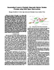
The reward measure includes components for both task completion and dialogue “appropriateness”, including: a reward of −100 for taking the greet action when not in the first turn of the dialogue; a reward of −3 for confirming a field before it has been referenced by the user; a reward of −5 for taking the fail action; a reward of +10 or −10 for taking the submit-x-y action when the user’s goal is (x,y) or not, respectively; and a reward of −1 otherwise. A discount of γ = 0.95 was used for all experiments. The initial (prior) probability of the user’s goal is distributed uniformly over the 6 user goals. Figure 1 shows an influence diagram of the POMDP.

5

the exponential probability density functions normalized to the region [0,1]; i.e., correct

correct

(19)

incorrect

incorrect

where acorrect and a incorrect are constants defined on (−∞, ∞) . We note that as a x approaches positive or negative infinity, p x (c) becomes deterministic and conveys complete information; when a x = 0 , p x (c) is a uniform density and conveys no information. Since we expect the confidence value for correct recognition hypotheses to tend to 1, and for incorrect recognition hypotheses to tend to 0, we would expect a x > 0 . 6

u

(18)

We define c on the interval [0,1] and define the probability densities p correct (c) and pincorrect (c ) as

 a correct e c⋅a , a correct ≠ 0  a −1 p correct (c) =  e   1, a correct = 0  aincorrect e (1−c ) a , aincorrect ≠ 0  ea −1 pincorrect (c) =   1, aincorrect = 0 

∑ p( s′ | s , a

su ∈Su

(16)

As noted above, the observation function accounts for the corruption introduced by the speech recognition engine, so we assume the observation depends only on the action taken by the user:6 p(h′, c′ | su′ , s′d , au′ , am ) = . p(h′, c′ | au′ ) = p(h, c | au )

b′( su′ , s′d , au′ ) = k ⋅ p(h′, c′ | au′ ) ⋅ p(au′ | su′ , am ) ⋅

In the testbed problem, we assume that the same recognition grammar is always used.

5.1

Comparison with MDP baseline Description of MDP baseline

To test whether the method for incorporating confidence score outperforms current methods, we created an MDP-based dialogue manager baseline, patterned on systems in the literature, such as (Pietquin, 2004). The MDP is trained and evaluated through interaction with a model of the environment, which is formed of the POMDP transition, observation, and reward functions. An MDP state estimator maps observations from the environment model to an MDP state. The confidence score is divided into M buckets. Ideally the confidence score bucket sizes would be selected so that they maximize average return. However, it is not obvious how to perform this selection – indeed, this is one of the weaknesses of “confidence bucket” method. Instead, a variety of techniques for setting confidence score threshold were explored. It was found that dividing the probability mass of the confidence score c evenly between buckets produced the largest average returns among the techniques explored. That is, we define cThresh0 = 0 < cThresh1 < L < cThreshM −1 < cThreshM = 1

and then find the values of cThreshm such that:

(21)

r

r'

su

su' sd

sd'

au

am

au'

{o,c}

am'

{o',c'}

Timestep n

Timestep n+1

Figure 1: Influence diagram depiction of the testbed POMDP. Symbols are as defined in the text. The dotted box shows the composite POMDP state, s. Note that the system action am depends on the belief state b(s) – the distribution over all states – and not the true current (unobservable) state. cThreshm

∫

p (c) dc =

cThreshm−1

cThreshm+1

∫ p(c) dc,

m ∈1,2,..., M − 1

(22)

cThreshm

where p(c) is the prior probability of a confidence score. We find this prior for our testbed problem as follows. We first find the distribution p(c | a u ) as: p(c | au ) =

∑ p(h, c | a ) u

(23)

h∈A

= pcorrect (c | au )(1 − perr ) + pincorrect (c | au )( perr ).

(24)

In the MDP context, we assume the confidence score buckets are formed without access to a prior p(a u ) . From this assumption, we find: p(c) = p correct (c)(1 − p err ) + pincorrect (c)( p err )

(25)

from which the values of cThreshm can be derived. The MDP state contains components for each field which reflect whether, from the standpoint of the machine, (a) a value has not been observed, (b) a value has been observed but not confirmed, or (c) a value has been confirmed. The MDP state also tracks which confidence bucket was observed for each field, as well as for the confirmation. Finally, two additional states – dialogue-start and dialogue-end – are included in the MDP state space. Because the confidence bucket for each field (including its value and its confirmation) is tracked in the MDP state, the size of the MDP state space grows with the number of confidence buckets. For M=2, the resulting MDP called MDP-2 has 51 states.7

7

For reference, M=1 produces an MDP with 11 states, and M=3 produces an MDP with 171 states.

Given the current MDP state, the MDP policy selects an MDP action, and the MDP state estimator then maps the MDP action back to a POMDP action. Because the MDP learns through experience with a simulated environment, an on-line learning technique, Watkins (1989) Q-learning, was used to train the MDP baseline. A variety of learning parameters were explored, and the best-performing parameter set was selected: initial Q values set to 0, exploration parameter ε = 0.2 , and the learning rate α set to 1/k (where k is the number of visits to the Q(s,a) being updated.). MDP-2 was trained with approximately 125,000 dialog turns. To evaluate the resulting MDP policy, 10,000 dialogs were simulated using the learned policy. 5.2

Results

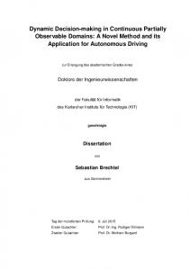
Both the Perseus and the Hoey-Poupart algorithms required two parameters for operation: number of belief points, and number of iterations. Through experimentation, we found that 500 belief points and 30 iterations attained asymptotic performance for all values of perr . In addition, the Hoey-Poupart algorithm required a parameter specifying the number of observations to sample at each belief point. Through experimentation, we found that 300 samples produced acceptable results and reasonable running times. Figure 2 shows the average returns for the continuous-POMDP, discrete-POMDP, and MDP-2 solutions vs. perr ranging from 0.00 to 0.65 for a correct = a incorrect = a = 1 . The error bars show the 95% confidence interval for return assuming a normal distribution. Note that return decreases consistently as perr increases for all solution methods, but the POMDP solutions attain larger returns than the MDP method at all values of perr .8 We next explored the effects of varying the informativeness of the confidence score. Figures 3, 4, and 5 show average returns for the two POMDP methods and MDP-2 method vs. a for perr = 0.3, 0.4, and 0.5, respectively. The error bars show the 95% confidence interval for return assuming a normal distribution. In these figures, we again define a correct = a incorrect = a . The POMDP methods outperform the baseline MDP method consistently. Note that increasing a increases average return for all methods, and that the greatest improvements are for p err = 0.5 – i.e., the information in the confidence score has more impact as speech recognition accuracy degrades.

8 The MDP-3 system was also created but we were unable to obtain better performance from it than we did from the MDP-2 system.

4

10 disc-POMDP MDP-2 cont-POMDP

6

3 2 Average return

Average return

8

4 2 0 -2

-4

0. 60 0. 65

0. 55

0. 45 0. 50

0. 40

0. 30 0. 35

0. 20 0. 25

0. 15

0. 05 0. 10

0. 00

disc-POMDP cont-POMDP MDP-2

-3

-6

0

perr

In Figures 2 through 5, the discrete-POMDP and continuous-POMDP methods performed similarly. This trend could be due to the relatively short horizon in the testbed problem: most of the dialogues spanned a handful of turns. Alternatively, this trend might indicate that the discrete-POMDP method provides sufficient planning. We intend to explore this issue with larger dialogue management problems in future work. 6 5.5 5 4.5 4 3.5 3 2.5

cont-POMDP MDP-2 disc-POMDP

2 1.5 1 0

1

2

5

a (Informativeness of confidence score)

Figure 3: Average return vs. a (informativeness of confidence score) at perr = 0.30 for continuous-POMDP, discrete-POMDP, and MDP-2 methods. 5 4 3 2 1 disc-POMDP cont-POMDP MDP-2

0 -1 0

1

1

2

5


Figure 2: Average return for continuous-POMDP, discrete-POMDP, and MDP-2 methods for a = 1.

Average return

0 -1 -2

-4

Average return

1

2

5


Figure 4: Average return vs. a (informativeness of confidence score) at perr = 0.40 for continuous-POMDP, discrete-POMDP, and MDP-2 methods.

Figure 5: Average return vs. a (informativeness of confidence score) at perr = 0.50 for continuous-POMDP, discrete-POMDP, and MDP-2 methods.

6

Improving handcrafted policies

In this section, we describe a method for improving a handcrafted policy by incorporating the belief state monitoring outlined above. Intuitively, a policy specifies what action to take in a given situation. In the previous section, we relied on the representation of a POMDP policy produced by value iteration – i.e., a value function, represented as a set of N vectors each of dimensionality |S|. We write υ n (s ) to indicate the sth component of the nth vector. Each vector represents the value, at all points in belief space, of executing some “policy tree” which starts with an action associated with that vector. We write πˆ (n) ∈ A to indicate the action associated with the nth vector. If we assume that the policy trees have an infinite horizon, then we can express the optimal policy at all timesteps as:   

S

  

π (b) = πˆ  arg max ∑υ n ( s) b( s )  n

s =1

(26)

Thus the value-function method provides both a partitioning of belief space into regions (each corresponding to an action which is optimal in that region), as well as the expected return of taking that action. A second way of representing a POMDP policy is as a “policy graph” – a finite state controller consisting of N nodes and some number of directed arcs. Each controller node is assigned a POMDP action, and we will again write πˆ (n) to indicate the action associated with the nth node. Each arc is labelled with a POMDP observation, such that all controller nodes have exactly one outward arc for each observation. l (n, o) denotes the successor node for node n and observation o. A policy graph is a general and common way of representing handcrafted dialogue management policies. More complex handcrafted policies – for example, those

created with rules – can usually be compiled into (possibly very large) policy graphs. We believe that a policy graph is a much more intuitive way for a human designer to specify a dialogue manager than a value function. 6.1

Method

To improve the policy graph, we will first need to evaluate it. Although a policy graph does not make the expected return associated with each controller node explicit, as pointed out by Hansen (1998), we can find the expected return associated with each controller node by solving this system of linear equations in υ :

υ n ( s ) = r ( s, πˆ (n)) +

γ ∑∑ p( s′ | s, πˆ (n)) p(o | s′, πˆ (n))υl ( n,o ) ( s′).

(27)

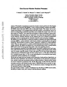
tion greet. HC1 takes the ask-from and ask-to actions to fill the from and to fields, performing no confirmation. If the user does not respond, it re-tries the same action. If it receives an observation which is inconsistent or nonsensical, it re-tries the same action. If it fills both fields without receiving any inconsistent information, it takes the corresponding submit-x-y action. A logical diagram showing HC1 is shown in .9

greet to Y from X

else

else

ask from

X from X

s′∈S o∈O

ask to

from X to Y

else

else

Y, to Y from X to Y, X≠Y

Solving this set of linear equations yields a set of vectors – one vector for each controller node. To find the expected value of starting the controller in node n and belief state b we compute:

from X to Y

guess X-Y

ask from

X from X from X to Y, X≠Y

Figure 6: HC1 handcrafted controller

S

∑υ ( s ) b ( s ) n

(28)

s =1

To improve the performance of the controller, we use υ n (s ) at run-time, as follows. At the beginning of the dialog, we find the node with the highest expected return for b0 and execute its action. Throughout the dialog, we perform belief state monitoring – i.e., we maintain the current belief state at each time-step as given in Eq. 3. At each time-step, rather than following the policy specified by the finite state controller, we reevaluate which node has the highest expected return for the current b. We then take the action specified by that node. Because the node-value function and belief state are exact, this style of execution is guaranteed to perform at least as well as the original handcrafted controller. Note that, in this style of execution, transitions may occur which are not arcs in the handcrafted policy. This style of execution is distinct from policy iteration, in which the nodes and links of the controller are changed and the controller is re-evaluated (using e.g., Eq 27) to iteratively improve the controller’s expected return. We do not explore policy iteration in this paper; however, we note that a handcrafted controller could be used to bootstrap a policy iteration process. Since a finite state controller is more intuitive for a (human) designer to understand, we intend to explore policy iteration in future work. 6.2

Testbed handcrafted controllers

Three handcrafted policies were created for the testbed dialogue management problem, called HC1, HC2, and HC3. All of the handcrafted policies first take the ac-

HC2 is identical to HC1 except that if the machine receives an observation which is inconsistent or nonsensical, it immediately takes the fail action. Once it fills both fields, it takes the corresponding submit-x-y action. HC3 employs a similar strategy to HC1 but extends HC1 by confirming each field as it is collected. If the user responds with “no” to a confirmation, it re-asks the field. If the user provides inconsistent information, it treats the new information as “correct” and confirms the new information. If the user does not respond, or if the machine receives any nonsensical input, it re-tries the same action. Once it has successfully filled and confirmed both fields, it takes the corresponding submit-x-y action. 6.3

Results

We first studied the operation of the greedy improvement method without access to confidence score information. We executed 10,000 dialogs for each handcrafted policy at values of perr ranging from 0.05 to 0.65. gives results for HC1. To make the gain of the greedy improvement method explicit, Figure 7 shows the difference between the proposed method and the expected value of executing the handcrafted policy directly. For reference, also includes the difference between the handcrafted policies executed normally and the POMDP policy, which we take to be a practical upper bound for the testbed problem. Error bars show the 95% confidence interval for the true expected return 9 A logical diagram is shown for clarity: the actual controller uses the real values a, b, and c, instead of the variables X and Y, resulting in a controller with 15 states.

Acknowledgements This work was supported in part by European Union Framework 6 TALK Project (507802).

Average or expected gain

0.6 0.4 0.2

0. 00 0. 05 0. 10 0. 15 0. 20 0. 25 0. 30 0. 35 0. 40 0. 45 0. 50 0. 55 0. 60 0. 65

Figure 7: Gain in average/expected return for HC1 executed using belief state monitoring vs. perr for a=0. (The POMDP policy, which we take to be our practical upper bound, is shown for reference in Figures 7 through 9.) 2.5 POMDP - HC2 HC2vf - HC2

2 1.5 1 0.5

0. 65

0. 55 0. 60

0. 50

0. 40 0. 45

0. 35

0. 30

0. 25

0. 20

0. 15

0. 10

0. 05

0. 00

0

perr

Figure 8: Gain in average/expected return for HC2 executed using belief state monitoring vs. perr for a=0. 5 4 3 2 1 POMDP - HC3 HC3vf - HC3

0

0. 65

0. 60

0. 50 0. 55

0. 45

0. 40

0. 35

0. 30

0. 25

0. 20

0. 10 0. 15

-1 0. 05

This work has shown how a confidence score can be directly incorporated into the dialogue model represented as a Partially Observable Markov Decision Process (POMDP) used for dialogue management. Through a testbed dialogue management problem, we have shown how recent optimization techniques are able to find policies which outperform traditional MDP approaches. Further, we have shown how handcrafted controllers can be automatically improved by performing belief state monitoring using confidence score information. This paper has focused on confidence score, but this technique could be used for other observable, continuous metrics with similar properties. In future work, we plan to incorporate “the speech recognition N-Best list” (i.e., a list comprised of N recognition hypotheses produced by the speech recogniser, each with an associated confidence score), as this should improve the quality of the belief state estimate. This extension would require altering the observation function to cope with a much larger observation space. However, this growth should not impact the amount of time required to optimize POMDP policies of a bounded size since the Hoey-Poupart (2005) method scales independently of the complexity of observation spaces for bounded-size policies. More broadly, we intend to scale up the model to handle larger problems. A method of exploiting redundancy in the model is needed to apply the method to domains with 100s or 1000s of concepts.

0.8

perr


Conclusions

POMDP-HC1 HC1vf-HC1

1

0


7

1.2

0. 00

assuming normal distribution. We note that in almost all cases, the greedy improvement method results in a significant improvement. In many cases, the improved handcraft controller is close to the POMDP policy – our assumed practical upper bound. Results for HC2 and HC3 are shown in Figures 8 and 9. We next studied the operation of the greedy improvement method when confidence score information is present. Figures 10, 11, and 12 show average returns for the discrete-POMDP and improved handcraft methods vs. a for perr = 0.3, 0.4, and 0.5, respectively. a is defined as in Section 5.2 – i.e., a = a correct = a incorrect . Error bars are negligible and are not shown. For each of the 3 handcrafted controllers in each of the 3 values of perr , increasing a consistently increases average return.

perr

Figure 9: Gain in average/expected return for HC3 executed using belief state monitoring vs. perr for a=0.

6

References

Average return

5

Eric A. Hansen. 1998. Solving POMDPs by searching in policy space. In Uncertainty in Artificial Intelligence, Madison, Wisconsin.

4 3 disc-POMDP HC2 HC1 HC3

2 1 0 0

1

2

5


Figure 10: Average return vs. a (informativeness of confidence score) for perr = 0.30 for discrete-POMDP and handcrafted policies executed with belief state monitoring.

4 Average return

Leslie Pack Kaelbling, Michael L. Littman and Anthony R. Cassandra. 1998. Planning and Acting in Partially Observable Stochastic Domains. Artificial Intelligence, Vol. 101. Esther Levin, Roberto Pieraccini, and Wieland Eckert. 2000. A Stochastic Model of Human-Machine Interaction for Learning Dialogue Strategies. IEEE Transactions on Speech and Audio Processing, Volume 8, No. 1, 11-23.

5

3 2 1

disc-POMDP HC2 HC1 HC3

0 -1 -2 0

1

2

5



Esther Levin and Roberto Pieraccini. 1997. A Stochastic Model of Computer-Human Interaction for Learning Dialogue Strategies. Eurospeech, Greece. Tim Paek and Eric Horvitz. 2003. On the Utility of Decision-Theoretic Hidden Subdialog. In Proceedings of International Speech Communication Association (ISCA) Workshop on Error Handling in Spoken Dialogue Systems, Switzerland. Olivier Pietquin. 2004. A Framework for Unsupervised Learning of Dialogue Strategies. Ph D thesis, Faculty of Engineering, Mons, Belgium. Nicholas Roy, Joelle Pineau and Sebastian Thrun. 2000. Spoken Dialogue Management Using Probabilistic Reasoning. Annual meeting of the Association for Computational Linguistics (ACL-2000).

4 3 2 Average return

Jesse Hoey and Pascal Poupart. 2005. Solving POMDPs with continuous or large observation spaces. To appear in Proceedings of the Joint International Conference on Artificial Intelligence (IJCAI), Edinburgh, Scotland.

1 0 -1

disc-POMDP HC2 HC1 HC3

-2 -3 -4 0

1

2

5



Satinder Singh, Diane Litman, Michael Kearns and Marilyn Walker. 2002. Optimizing Dialogue Management with Reinforcement Leaning: Experiments with the NJFun System. Journal of Artificial Intelligence, Vol. 16, 105-133. Matthijs T. J. Spaan and Nikos Vlassis. 2004. Perseus: randomized point-based value iteration for POMDPs. Technical Report IAS-UVA-04-02, Informatics Institute, University of Amsterdam. C. J. C. H. Watkins. 1989. Learning from Delayed Rewards. Ph.D. thesis, Cambridge University. B. Zhang, Q. Cai, J. Mao, E. Chang, and B. Guo. 2001. Spoken Dialogue Management as Planning and Acting under Uncertainty. Eurospeech. Denmark.