which have logarithmic output energy of Mel-filter bank of ob- served noisy speech, clean ..... ing clean training data of AURORA-2J with several states and mix-.
➠
➡ PARTICLE FILTER BASED NON-STATIONARY NOISE TRACKING FOR ROBUST SPEECH RECOGNITION Masakiyo Fujimoto and Satoshi Nakamura ATR Spoken Language Translation Research Laboratories 2-2-2, Hikari-dai, Seika-cho, Souraku-gun, Kyoto, 619-0288, Japan E-mail: {masakiyo.fujimoto, satoshi.nakamura}@atr.jp ABSTRACT This paper addresses the main speech recognition problem in nonstationary noise environments: the estimation of noise sequences. To solve this problem, we present a particle filter-based sequential noise estimation method for front-end processing of speech recognition in noise. In the proposed method, a noise sequence is estimated through a sequential importance sampling step, then a residual resampling step, and finally a Markov chain Monte Carlo step with Metropolis-Hastings sampling. The estimated noise sequence is applied to MMSE-based clean speech estimation method. The evaluations were conducted on speech recognition in highly nonstationary noise environments. In the evaluation results, we observed that the proposed method improves speech recognition accuracy in non-stationary noise environments over noise compensation with stationary noise assumptions. 1. INTRODUCTION Noise robustness is one of the most important problems for the applications of speech recognition techniques in real environments. For this problem, when adverse noise is restricted to stationary noise, a lot of research in speech recognition in noise has been reported [1]-[4]. However, most of the noise observed in real environments have non-stationary characteristics. To improve the speech recognition accuracy in non-stationary noise environments, it is necessary to estimate the noise sequence as accurately as possible. However, the estimation of non-stationary noise sequences is difficult because, in most cases, the observable signal when speech recognition is performed is the only noise added to the speech signal. So both clean speech and noise have non-stationary characteristics. To solve such problems, several estimation methods of nonstationary noise sequences based on a sequential EM algorithm are reported [5]-[7], that can estimate noise sequence effectively. However, their computation costs are expensive because frame by frame iterative estimation is required to converge noise parameters. Recently, a particle filter-based sequential estimation method [8, 9] has attracted attention and been applied to various research fields. The particle filter is a Bayesian estimation method, whose main estimation framework is based on a sequential Monte-Carlo method. Therefore, the computation costs of the particle filter are cheaper than a sequential EM algorithm because iterative estimation is not required. In this paper, we present a sequential non-stationary noise estimation method based on a particle filter. In the proposed method, the sequence of non-stationary noise is estimated through extended Kalman filter-based sequential importance sampling, residual re-
0-7803-8874-7/05/$20.00 ©2005 IEEE
sampling, and a Markov chain Monte Carlo with Metropolis-Hastings sampling. Then, noise estimation is carried out frame by frame, and the estimated noise sequence is applied to a minimum mean square error (MMSE)-based clean speech estimation method [2]. A particle filter-based method similar to our proposed method was also reported by Yao et al [9]. Yao’s approach is an HMM composition-based acoustic model compensation method which updates an acoustic model sequentially by using estimated noise. On the other hand, our approach is a noise compensation method for front-end processing of speech recognition. Therefore, our method can carry out such multiple stage processing as a combination of front-end noise suppression and acoustic model adaptation for residual noise caused by front-end processing. Moreover, in a HMM composition method, a noise-compensated HMM is composed by using a clean speech HMM and a noise HMM. Generally, both clean speech and noise HMMs used for a HMM composition method are trained by using data without cepstral mean subtraction (CMS). Therefore, a HMM composition method cannot be applied to the CMS for the testing (observation) data. On the other hand, the proposed method can be applied to CMS to estimated clean speech because it is a noise compensation method for front-end processing, and the acoustic model is trained by using estimated clean speech after CMS processing. Our proposed method was evaluated on a connected Japanese digits recognition task [10], conducted on speech recognition in highly non-stationary noise environments. In the evaluation results, we observed that the proposed method improves speech recognition accuracy in non-stationary noise environments over noise compensation with stationary noise assumptions. 2. PARTICLE FILTER-BASED NOISE ESTIMATION 2.1. Dynamical system for noise sequence A dynamical system can be defined by two equations: a state transition equation that represents the dynamics of the target signal, and an observation equation that represents the output system of the observed signal. Let Xt , St , and Nt denote the vectors at t-th short time frame which have logarithmic output energy of Mel-filter bank of observed noisy speech, clean speech, and noise, respectively. The dynamical system for noise sequence is represented as follows. First, assume that clean speech St can be modeled by a hidden Markov model (HMM). At time t parameter Sst ,kt ,t is generated from a Gaussian distribution kt contained in state st of clean speech HMM. In this case, the observation process of Xt can be modeled by the following equation by using Nt and error signal Vt ,
I - 257
ICASSP 2005
➡
➡ (j)
Xt
= =
sample weight wt can be represented as a following recursive formula by substituting Eq. (9) and Eq. (8) into Eq. (7):
Sst ,kt ,t + log (I + exp (Nt − Sst ,kt ,t )) + Vt f (Sst ,kt ,t , Nt ) + Vt (1) Vt ∼ N (0, ΣS,st ,kt ),
(j)
wt
(2)
(j)
wt where
(4)
(j)
(j)
Kt
ˆ t(j) N
(j)
(j)
st
st
p(Nt |Nt−1 )p(Xt |Nt ) p(N0:t−1 |X0:t−1 ) p(Xt |X0:t−1 ) (8) ∝ p(Nt |Nt−1 )p(Xt |Nt )p(N0:t−1 |X0:t−1 ).
Furthermore, if importance density q(N0:t |X0:t ) has the following recursive formula, q(N0:t |X0:t ) = q(Nt |N0:t−1 , X0:t )q(N0:t−1 |X0:t−1 ),
(9)
,kt
(j)
st
«
« , ΣS,s(j) ,k(j) t
t
.
(13)
(j)
=
(j) ΣNt|t−1
,kt
−
,kt
,t
(j) (j) (j) Kt Ft ΣNt|t−1 ,
(18)
,t
,t
t
∼ aS,s(j)
(j)
t
t
t−1 st
t
(j)
t−1 st
where µS,s(j) ,k(j) , aS,s(j)
where q(N0:t |X0:t ) ∝ p(N0:t |X0:t ). By applying a Bayesian rule to Eq. (5), a posteriori PDF with a recursive formula for obtaining p(N0:t |X0:t ) from p(N0:t−1 |X0:t−1 ) is given by p(N0:t |X0:t ) =
(j)
, Nt
from clean speech HMM as follows: “ ” (j) S (j) (j) ∼ N µS,s(j) ,k(j) , ΣS,s(j) ,k(j)
(7)
(j)
(j) ,kt ,t
(11)
where subscript t|t−1 denotes the predicted parameter from t−1(j) th frame and S (j) (j) denotes the clean speech samples drawn
(j)
q(N0:t |X0:t )
(j)
st
(j) ΣNt−1
and δ(·) denote sample index, the number of where j, J, P (j) samples, weight of sample j at time t ( Jj=1 wt = 1), and a Dirac delta function, respectively. When direct sampling from p(N0:t |X0:t ) is intractable, we can draw the samples from the other distribution q(N0:t |X0:t ), which is related to p(N0:t |X0:t ) and called an importance density. (j) Therefore, when samples N0:t were drawn from the importance (j) (j) density q(N0:t |X0:t ), sample weight wt is defined as ,
(j)
(14) ΣNt|t−1 = ΣNt−1 + ΣW h i−1 (j) (j)T (j) (j) (j)T = ΣNt|t−1 Ft + ΣS,s(j) ,k(j) Ft ΣNt|t−1 Ft t t (15) „ «. (j) (j) (j) (j) Ft = ∂f S (j) (j) , Nt|t−1 (16) ∂Nt|t−1 st ,kt ,t „ „ «« (j) (j) (j) (j) = Nt|t−1 + Kt Xt − f S (j) (j) , Nt|t−1 (17)
(j) wt ,
p(N0:t |X0:t )
(j)
(j) (j) ˆ t−1 Nt|t−1 = N
j=1
∝
(j)
st
p(Nt� |Nt� −1 )p(Xt� |Nt� ), (5)
where N0:t = {N0 , . . . , Nt } and X0:t = {X0 , . . . , Xt }. Therefore, N0:t is estimated as the signal which recursively maximizes the above PDF. In a particle filtering algorithm, a posteriori PDF p(N0:t |X0:t ) is approximated by Monte Carlo sampling as follows: J “ ” X (j) (j) p(N0:t |X0:t ) � wt δ N0:t − N0:t , (6)
(j)
(10)
2.3. Parameter updating by extended Kalman filter (j) (j) To update the noise samples Nt from previous samples Nt−1 , an extended Kalman filter, which is derived by the dynamical system defined by Eqs. (1) and (3), is applied. The extended Kalman filterbased updating formula is given by
t� =1
wt
(j)
.
(12) Generally, the above particle filtering algorithm is called a sequential importance sampling (SIS) particle filter [8].
2.2. Sequential importance sampling for particle filtering When a dynamical system derived by Eqs. (1) and (3) is given, a posteriori probability density function (PDF) for the sequence of Nt can be represented by a first order Markov chain as follows: t Y
(j)
∝ wt−1 p(Xt |Nt ),
„ „ (j) Xt ; f S (j)
(j)
p(Xt |Nt ) = N
where Wt and ΣW denote the driving noise for state transition process and diagonal covariance matrix of Wt , respectively.
p(N0:t |X0:t ) = p(N0 |X0 )
(j)
(j) (j) q(Nt |N0:t−1 , X0:t ) (j)
(3)
Wt ∼ N (0, ΣW ),
(j)
p(Nt |Nt−1 )p(Xt |Nt )
In Eq. (10), we assumed that p(Nt |Nt−1 ) = q(Nt |N0:t−1 , X0:t ). Therefore, it is simplified as
where ΣS,st ,kt denotes the diagonal covariance matrix of Gaussian distribution contained in clean speech HMM. On the other hand, we assumed that the state transition process of Nt can be modeled by a random walk process as follows: Nt = Nt−1 + Wt
(j)
∝ wt−1
, kt
t
t
∼ PS,s(j) ,k t
(19) (20)
t
, and PS,s(j) ,k denote the mean vect
t
(j)
tor of kt -th Gaussian distribution contained in state st of clean (j) speech HMM, state transition probability from st−1 to st , and mixture weight, respectively. Initial noise samples are drawn as (j)
(j)
N0 ∼ N (µN , ΣN ) , ΣN0 = ΣN , (21) where µN and ΣN denote mean vector and diagonal covariance matrix of initial noise distribution, respectively. µN and ΣN are estimated by using the first 10 frames of observations. 2.4. Residual resampling (selection) step In practice, after the sampling step described in Section 2.2, the weights of all but several samples may become insignificant. Given the fixed number of samples, this will degenerate the estimation. A selection step by residual resampling [8] is adopted after the sampling step. Figure 1 illustrates the summary of residual resampling step.
I - 258
➡
➡ The method avoids degeneracy by discarding those samples with insignificant weights, and to keep the number of samples constant, samples with significant weights are duplicated. Accordingly, the weights after the selection step are also proportionally redistributed. Noise distribution
Sampling t Selection Sampling t+1
: Sample with large weight : Sample with small weight
Selection
Fig. 1. Summary of residual resampling step 2.5. Markov chain Monte Carlo step After the resampling step at frame t, these J samples are distributed approximately according to Eq. (6). However, the discrete nature of the approximation can skew the importance weights distribution, where in extreme cases all the samples have the same value. A Metropolis-Hastings (MH) sampling [11] step is introduced in each sample where the step involves sampling a candidate given the current state according to proposal importance distribution. To simplify the calculation, we assume that the importance distribution is symmetric. After some mathematical manipulation, it is shown that an acceptance possibility is given by n o ∗(j) (j) ν = min 1, wt /wt , (22) ∗(j)
denotes sample weight computed by MH sampling where wt step. The state transition by MH sampling is derived as: ( ∗(j) if u ≤ ν (accept state transition) Nt (j) , Nt = (j) otherwise (reject state transition) Nt (23) ∗(j) where Nt denotes samples drawn by MH sampling step and u ∼ U[0,1] . U[0,1] is the uniform distribution between 0 and 1.
ˆ t is given by Finally, a clean speech estimate S J X (j) (j) ˆt = ˆt . S wt S
3. EXPERIMENTS 3.1. Experimental setup Speaker independent Japanese connected digits recognition were carried out by using HTK ver.3.2. 8440 connected digits utterances spoken by 110 speakers and 1001 connected digits utterances spoken by 104 speakers were used for training and testing. These materials were taken from AURORA-2J [10]. Factory and road working noises were artificially added to clean testing data with various SNRs from 0dB to 20dB. The feature parameters used in this evaluation were composed of 39 MFCCs with 13 MFCCs (with zero-th MFCC) and their first and second order derivatives. A zero-th MFCC was used as energy coefficient instead of a standard Log-energy. At the feature extraction stage, CMS was applied to each sentence. AURORA-2J standard whole word HMMs (16 states, 20 mixture distributions per state) were used for speech recognition. We also trained the clean speech HMM for noise compensation by using clean training data of AURORA-2J with several states and mixture distributions: namely, 1 state model (512 mixtures per state), 4 states model (128 mixtures per state), 8 states model (64 mixtures per state), and 16 states model (32 mixtures per state). The number of distributions contained in an HMM were 512 for all HMMs. The feature parameters were 23th order log output energy of Melfilter bank. In particle filter-based noise estimation, the number of samples was set to 20, and the covariance matrix of driving noise Wt was set to ΣW = diag(0.01). 3.2. Experimental results Figure 2 illustrates the estimation results of factory noise. In the figure, “True noise,” “Moving average,” and “Particle filter” indicate the true noise sequence of the first log output energy of a Mel-filter bank, the sequence of “True noise” smoothed by moving average with 20 frame intervals, and, noise sequence estimated by our proposed method with a 16 state HMM, respectively. The processing performance of the proposed method with a 16 state HMM was about 0.8 times that of real time by a 3.2GHz Intel Xeon processor.
2.6. MMSE estimation of clean speech We estimated clean speech St by using MMSE estimation [2]. Clean speech estimates with one noise sample are given by the following MMSE formula: K “ “ ”” X (j) ˆ (j) S = Xt − P (k|Xt , (j)) log I + exp Nt − µS,s(j) ,k , t
㪣㫆㪾㩷㫆㫌㫋㫇㫌㫋㩷㪼㫅㪼㫉㪾㫐㩷㫆㪽㩷㪤㪼㫃㩷㪽㫀㫃㫋㪼㫉㩷㪹㪸㫅㫂
㪏
t
k=1
(24) where K denotes the number of mixtures and P (k|Xt , (j)) is given by „ « PS,s(j) ,k N Xt , µX(j) , ΣX(j) t k,t k,t „ «, P (k|Xt , (j)) = PK P N X , µ , Σ (j) (j) (j) t � k =1 S,s ,k� X X k� ,t
t
k� ,t
(25) where µX(j) and ΣX(j) denote mean vector and diagonal covarik,t
k,t
ance matrix of Xt which are compensated by first order VTS(j) based approach [4] with parameters µS,s(j) ,k , ΣS,s(j) ,k , Nt and (j)
ΣNt .
t
t
(26)
j=1
㪫㫉㫌㪼㩷㫅㫆㫀㫊㪼 㪤㫆㫍㫀㫅㪾㩷㪸㫍㪼㫉㪸㪾㪼 㪧㪸㫉㫋㫀㪺㫃㪼㩷㪽㫀㫃㫋㪼㫉
㪎㪅㪌
㪎
㪍㪅㪌
㪍
㪌㪅㪌
㪌 㪈㪐
㪊㪐
㪌㪐
㪎㪐
㪐㪐
㪈㪈㪐
㪈㪊㪐
㪈㪌㪐
㪈㪎㪐
㪈㪐㪐
㪉㪈㪐
㪉㪊㪐
㪉㪌㪐
㪉㪎㪐
㪝㫉㪸㫄㪼㩷㫀㫅㪻㪼㫏
Fig. 2. Estimation results of factory noise by 16 states HMM Figure 2 shows that the estimated noise sequence is close to that of “Moving average”. However, the estimation accuracy was insufficient when abrupt changes occurred. Moreover, compared with “True noise”, estimation error was large throughout all noise sequences. This is caused by inaccurate modeling of dynamical
I - 259
➡
➠ Table 1. Word accuracy of factory noise environments (%) SNR 20 dB 15 dB 10 dB 5 dB 0 dB Average
HTK baseline 93.61 81.12 54.81 29.47 18.73 55.55
ETSI Advanced front-end 92.88 86.86 76.73 53.18 23.15 66.56
HTK baseline 96.68 89.93 70.28 38.81 22.29 63.60
ETSI Advanced front-end 96.90 94.81 89.81 76.02 48.48 81.20
MMSE (Stationary noise compensation) 96.41 88.92 74.27 50.94 24.72 67.05
1 state 96.04 89.59 75.41 51.98 26.19 67.84
Particle filter 4 states 8 states 95.03 95.82 87.38 88.82 72.95 73.90 51.30 50.54 28.55 26.50 67.04 67.12
16 states 96.13 90.02 75.87 54.50 28.92 69.09
Upper limit (True noise) 98.46 94.87 85.11 63.13 37.06 75.73
16 states 98.34 95.61 89.84 75.28 49.43 81.70
Upper limit (True noise) 99.29 98.16 94.87 82.69 54.51 85.90
Table 2. Word accuracy of road working noise environments (%) SNR 20 dB 15 dB 10 dB 5 dB 0 dB Average
MMSE (Stationary noise compensation) 99.20 97.61 91.77 71.57 43.60 80.75
system for noise. We employed a random walk process represented by Eq. (3) for a state transition process. However, a random walk process does not ensure the accurate state transition of noise. To reduce estimation error of noise sequences, it is necessary to investigate an accurate modeling method of noise dynamics. Tables 1 and 2 indicate the speech recognition results for word accuracy. In the tables, “HTK Baseline,” “ETSI Advanced frontend,” “MMSE,” and “Particle filter” indicate the recognition results without noise compensation, results by ETSI Advanced frontend [3], results by MMSE estimation with stationary noise compensation and 1 state model, and results by MMSE estimation with particle filter (non-stationary noise compensation), respectively. “Upper limit” indicates the results by MMSE estimation with true noise sequence and 1 state model. Tables 1 and 2 show that the proposed method with a 16 state model exhibits the best average word accuracy. However, the performance improvement from “MMSE” was small. To improve word accuracy, it is necessary to estimate noise sequences as accurately as possible, since the potential of MMSE with true noise sequence is large. As we can see from the tables, to improve the accuracy of noise estimation, we have to increase the number of states of clean speech HMMs. These results suggest that noise estimation accuracy by the proposed method depends not only on noise dynamics but also clean speech dynamics, because accurate clean speech samples are required to update the noise samples and compute the sample weight as shown in Sections 2.2 and 2.3. The reliabilities of clean speech samples depend on the modeling accuracy of clean speech HMMs. If a clean speech HMM has a large number of states, the reliabilities of clean speech samples will increase because an HMM with a large number of states can model the detailed dynamics of clean speech. From these facts, we have to consider the optimal modeling of clean speech HMMs for particle filter-based noise estimation. 4. CONCLUSION A particle filter-based non-stationary noise estimation method has been presented in this paper. In the evaluation results, the proposed method showed improvements of speech recognition accuracy in non-stationary noise environments. Furthermore, it showed that accurate dynamics modeling for both noise and clean speech is
1 state 98.34 97.08 92.39 73.04 43.44 80.86
Particle filter 4 states 8 states 97.85 98.46 95.21 96.07 88.79 90.33 72.24 74.21 48.88 46.88 80.59 81.19
an important factor for particle filter-based noise estimation. In the future, we are planning to investigate the accurate modeling of noise dynamics and the optimal modeling of clean speech HMM for particle filter-based noise estimation. 5. ACKNOWLEDGEMENTS This research was supported in part by the National Institute of Information and Communications Technology. The present study was conducted using a AURORA-2J database developed by the IPSJ-SIG SLP Noisy Speech Recognition Evaluation Working Group. 6. REFERENCES [1] S.F.Boll: “Suppression of Acoustic Noise in Speech Using Spectral Subtraction,” IEEE Trans. ASSP, Vol.27, No.2, pp.113-120, 1979. [2] J.C.Segura, A.de la Torre, M.C.Benitez, and A.M.Peinado: “ModelBased Compensation of the Additive Noise for Continuous Speech Recognition. Experiments Using AURORA II Database and Tasks,” EuroSpeech’01, Vol.I, pp.221-224, 2001. [3] ETSI ES 202 050 V1.1.1, “Distributed speech recognition; advanced front-end feature extraction algorithm; compression algorithms,” 2002. [4] P.J.Moreno, B.Raj, and R.M.Stern: “A Vector Taylor Series Approach for Environment-Independent Speech Recognition,” ICASSP’96, pp.733-736, 1996. [5] M.Afify and O.Siohan: “Sequential Estimation with Optimal Forgetting for Robust Speech Recognition,” IEEE Trans. SAP, Vol.12, No. 1, pp.19-26, 2004 [6] K.Yao, K.K.Paliwal, and S.Nakamura, “Noise adaptive speech recognition based on sequential noise parameter estimation,” Speech Communication, Vol.42, Issue 1, pp.5-23, 2004. [7] T.A.Myrvoll and S.Nakamura: “Optimal Filtering of Noisy Cepstral Coefficients for Robust ASR,” ASRU2003, pp.381-386, 2003. [8] M.S.Arulampalam, S.Maskell, N.Gordon, and T.Clapp: “A Tutorial on Particle Filters for Online Nonlinear/Non-Gaussian Bayesian Tracking,” IEEE Trans. SP, Vol.50, No.2, 2002. [9] K.Yao and S.Nakamura: “Sequential noise compensation by sequential Monte Carlo method,” NIPS2001, pp.1205-1212, 2001. [10] S.Nakamura, K.Yamamoto, K.Takeda, S.Kuroiwa, N.Kitaoka, T.Yamada, M.Mizumachi, T.Nishiura, M.Fujimoto, A.Sasou, and T.Endo: “Data Collection and Evaluation of AURORA2-J Japanese Corpus,” ASRU2003, pp.619-623, 2003. [11] W.K.Hastings: “Monte Carlo sampling methods using Markov chains and their applications,” Biometrika, Vol.57, pp.97-109, 1970.
I - 260