Process Noise Identification Based Particle Filter: an Efficient Method to Track Highly Maneuvering Target Liu Jing School of Electronics and Information Engineering, Xi’an JiaoTong University, Xi’an, P.R.China.
[email protected]
Han ChongZhao School of Electronics and Information Engineering, Xi’an JiaoTong University, Xi’an, P.R.China.
[email protected]
Abstract – In this paper, a novel method, process noise identification based particle filter is proposed for tracking highly maneuvering target. In the proposed method, the equivalent-noise approach [1], [2], [3] is adopted, which converts the problem of maneuvering target tracking to that of state estimation in the presence of non-stationary process noise with unknown statistics. A novel method for identifying the nonstationary process noise is proposed in the particle filter framework. Compared with the multiple model approaches for maneuvering target tracking, the proposed method needs to know neither the possible multiple models nor the transition probability matrices. One simple dynamic model is adopted during the whole tracking process. The proposed method is especially suitable for tracking highly maneuvering target due to its capability of dealing with sample impoverishment, which is a common problem in particle filter and becomes serious when tracking large uncertain dynamics. Keywords: Particle filter, process noise identification, maneuvering target tracking, sample impoverishment
1
Introduction
Particle filter, which uses sequential Monte Carlo methods for on-line learning within a Bayesian framework, can be applied to any state-space models. Particle filter is more suitable than Kalman filter and extended Kalman filter when dealing with non-linear and non-Gaussian estimation problems. The application of particle filter in maneuvering target tracking has been paid attention only in recent years [4, 5, 6, 7, 8, 9, 10, 11]. Recently, several approaches, which use multiple models to describe the changing maneuvering model, have been proposed in the particle filter framework. One of the methods is based on the auxiliary particle filter. In [6], Karlsson used an auxiliary particle filter to track a highly maneuvering target. In this method, each particle is split deterministically into a number
Prahlad Vadakkepat Department of Electrical and Computer Engineering, National University of Singapore, Singapore.
[email protected]
of possible maneuver hypotheses with each hypothesis corresponding to a specific model. Other methods focus on how to switch between different motion models. In [7], Bayesian switching structure is chosen as the principle which determines switching between different models. A set of models are utilized to cope with the unknown maneuver. Moreover, to deal with non-Gaussian noise, Cauchy distribution is used as the system noise distribution. In [8] and [9], the maneuvering target tracking system is treated as a jump Markov linear system. MCMC process is used as the selection scheme to choose the motion model from a set of candidate models at some specific time step. However, in the above approaches [6, 7, 8, 9], the possible motion models and transition probability matrices are assumed as known. In practice, the dynamics is hard to break up into several different motion models and the model transition probabilities are difficult to obtain. A general model is needed to cope with the wide variety of motions exhibited by the maneuvering target. For the single model based methods, Karlsson [16] and Ikoma [17] applied optimal recursive Bayesian filters directly to the nonlinear target model. Both the algorithms are based on the assumption of small amplitude of maneuvers and could not cope with large maneuvers. That reflects that the standard particle filter should be improved to deal with the wide variation of the maneuvering movement. The algorithm may fail due to sample impoverishment when tracking wide variation in maneuvering movements. In the generic particle filter algorithm, the optimal proposal distribution is 𝑝(𝑥𝑘 ∣𝑥𝑖𝑘−1 , 𝑧𝑘 ), which is based on both the previous state and the current measurements [12]. However, in the standard particle filter, the prior distribution 𝑝(𝑥𝑘 ∣𝑥𝑖𝑘−1 ) is chosen as the proposal distribution for simplicity. In the standard particle filter algorithm, at each time step the predicted particles are generated from the prior distribution and could not catch the latest variation of the state variables, espe-
cially when the target is carrying out large maneuvers induced by fast changing motion models. This might be due to the reason that the current measurements are not considered in the prior distribution. As a result, most of the particles are assigned with low weights and eliminated via the resampling process. This leads to serious sample impoverishment and then the tracking process fails. There have been some systematic techniques proposed recently to solve the problem of sample impoverishment. One such technique is regularized particle filter [18], which resamples from a continuous approximation of the posterior density of the target state, whereas the standard particle lter resamples from the discrete approximation of the posterior density. This approach is frequently found to improve performance, despite a less rigorous derivation. An alternative solution to the same problem is the resample-move algorithm [19]. This technique uses periodic MCMC steps to diversify particles in an importance sampling-based particle lter. It does so in a rigorous manner that ensures the particles asymtotically approximate samples from the posterior. However, the resample-move algorithm can not avoid sample impoverishment due to the existence of ressampling procedure at each time step. Moreover, the traditional MCMC sampling needs a lot of iterations to converge to the target posterior distribution, which is very slow and not suitable for real-time tracking. In this paper, a new method, named process noise identification based particle filter, is proposed to tackle the sample impoverishment problem. The proposed method is based on the assumption that the random effect (including maneuvers and random noises) can be modeled by (part of) a white or colored noise process sufficiently well. This fundamental assumption converts the problem of maneuvering target tracking to that of state estimation in presence of non-stationary process noise with unknown statistics. In order to identify the distribution of the process noise, a dynamic system is modeled with the process noise and measurement vectors as its state and measurement vectors respectively. A sampling based algorithm is then proposed in the particle filter framework to estimate the state vector (process noise) based on the current measurements. Using the newly obtained process noise samples, the predicted particles are generated easily from a single general dynamic model. In the proposed method, the predicted particles are generated indirectly from the current measurements through the process noise samples. The predicted particles are more close to the current state of the target, which can reduce the sample impoverishment effectively. The rest of the paper is organized as follows. In Section 2 the basic theory and procedure of particle filter for state estimation are provided. The process noise identification based particle filter algorithm for track-
ing highly maneuvering target is introduced in Section 3. The simulation results are shown in Section 4 and the paper is summarized in Section 5.
2
Basic Theory of Particle Filter
To define the problem of tracking, consider a dynamic system represented by the state equation: ∗ 𝑥𝑘 = 𝑓 (𝑥𝑘−1 , 𝑣𝑘−1 ),
(1)
where 𝑥 is the state, 𝑓 is a possibly nonlinear function, and 𝑣 ∗ is the known process noise with a zero mean Gaussian distribution. The objective of tracking is to recursively estimate 𝑥𝑘 from a sequence of measurements up to time step 𝑘, 𝑧1:𝑘 = {𝑧1 , 𝑧2 , ⋅ ⋅ ⋅ , 𝑧𝑘 }. The observation model is described as follows, 𝑧𝑘 = ℎ(𝑥𝑘 , 𝑛𝑘 ),
(2)
where ℎ is a possibly nonlinear function. 𝑛 is the observation noise with a zero mean Gaussian distribution. From the Bayesian perspective, the tracking problem is to recursively calculate the posterior distribution 𝑝(𝑥𝑘 ∣𝑧1:𝑘 ). In this paper, a particle filter is considered to solve the state estimation problem due to its ability to tackle the non-linear and non-Gaussian systems. The posterior distribution 𝑝(𝑥𝑘 ∣𝑧1:𝑘 ) is approximated by a set of particles with associated weights. The detailed introduction about particle filter algorithm can be found in [12]. The procedures associated with the standard particle filter are listed in the following: Algorithm 1: Particle Filter Algorithm (1) Initialization: Sample initial particles {𝑥𝑖0 , 𝑖 = 1, ..., 𝐻} from the initial posterior distribution 𝑝(𝑥0 ) 1 , 𝑖 = 1, ..., 𝐻. 𝐻 is the and set the weights 𝑤0𝑖 to 𝐻 number of particles. (2) Prediction: Particles at time step 𝑘 − 1, {𝑥𝑖𝑘−1 , 𝑖 = 1, ..., 𝐻}, are passed through the system model (3) to obtain the predicted particles at time step 𝑘, {ˆ 𝑥𝑖𝑘 , 𝑖 = 1, ..., 𝐻}: ∗,𝑖 𝑥 ˆ𝑖𝑘 = 𝑓 (𝑥𝑖𝑘−1 , 𝑣𝑘−1 ),
(3)
∗,𝑖 where 𝑣𝑘−1 is a sample drawn from the known zero mean Gaussian distribution. (3) Update: Once the observation data, 𝑧𝑘 , is measured, evaluate the importance weight of each predicted particle and obtain the normalized weight for each particle (4).
𝑤 ˆ𝑘𝑖 = 𝑝(𝑧𝑘 ∣ˆ 𝑥𝑖𝑘 ),
𝑤 ˆ𝑖 𝑤𝑘𝑖 = ∑𝐻 𝑘 𝑖=1
𝑤 ˆ𝑘𝑖
(4)
Thus at time can obtain the estimate of the ∑step 𝑘 we 𝑖 ˜˜𝑘 = 𝐻 𝑤𝑖 𝑥 state, 𝑥 𝑖=1 𝑘 ˆ𝑘 . (4) Resample : Resample the discrete distribution {𝑤𝑘𝑖 : 𝑖 = 1, ⋅ ⋅ ⋅ , 𝐻} 𝐻 times to generate particles {𝑥𝑗𝑘 :
𝑗 = 1, ⋅ ⋅ ⋅ , 𝐻}, so that for any 𝑗, 𝑃 𝑟{𝑥𝑗𝑘 = 𝑥 ˆ𝑖𝑘 } = 𝑤𝑘𝑖 . 1 𝑖 Set the weights 𝑤𝑘 to 𝐻 , 𝑖 = 1, ..., 𝐻, and move to Stage 2.
3
Maneuvering Target Tracking Based on Process Noise Identification
The general motion model of a maneuvering target can be described by the following state-space model, ∗ 𝑥𝑘 = 𝑓 (𝑥𝑘−1 , 𝑢𝑘−1 , 𝑣𝑘−1 ),
(5)
where 𝑢 is the maneuver acceleration and 𝑣 ∗ is the process noise. In the equivalent-noise approach [1], [2], [3], it is assumed that the equation (5) that describes target motions can be simplified to, 𝑥𝑘 = 𝑓 (𝑥𝑘−1 , 𝑣𝑘−1 ),
(6)
with an adequate accuracy, where 𝑣 is the equivalent noise that quantifies the error of this model in describing the target motions, in particular, maneuvers. The statistics of this noise 𝑣, non-stationary in general, are not known. In this section, a novel method is proposed for process noise identification. The process noise is modeled as a dynamic system. The noise vector 𝑣𝑘−1 is chosen as the state of the noise system. The observation vector is 𝑧𝑘 , which is same as in equation (2). The observation equation is defined in (7), 𝑧𝑘 = ℎ(𝑥𝑘 , 𝑛𝑘 ) = ℎ[𝑓 (𝑥𝑘−1 , 𝑣𝑘−1 ), 𝑛𝑘 ].
(7)
The aim of the proposed method is to estimate the posterior distribution of the process noise, 𝑝(𝑣𝑘−1 ∣𝑧1:𝑘 ). According to the Bayesian inference theory, 𝑝(𝑣𝑘−1 ∣𝑧1:𝑘 ) =
𝑝(𝑧𝑘 ∣𝑣𝑘−1 )𝑝(𝑣𝑘−1 ∣𝑧1:𝑘−1 ) , 𝑝(𝑧𝑘 ∣𝑧1:𝑘−1 )
(8)
where 𝑝(𝑧𝑘 ∣𝑧1:𝑘−1 ) is a normalizing constant and 1 𝑝(𝑧𝑘 ∣𝑧1:𝑘−1 ) is defined as Υ. So we can obtain 𝑝(𝑣𝑘−1 ∣𝑧1:𝑘 ) = Υ ⋅ 𝑝(𝑧𝑘 ∣𝑣𝑘−1 )𝑝(𝑣𝑘−1 ∣𝑧1:𝑘−1 ).
(9)
The noise 𝑣𝑘−1 may be from random accelerations, sudden maneuvers or both, and there is no information about the distribution of 𝑣𝑘−1 . 𝑣𝑘−1 is not dependent on the previous measurements 𝑧1:𝑘−1 , which results in (10), 𝑝(𝑣𝑘−1 ∣𝑧1:𝑘 ) = Υ ⋅ 𝑝(𝑧𝑘 ∣𝑣𝑘−1 )𝑝(𝑣𝑘−1 ).
(10)
Since there is no information about 𝑣𝑘−1 , it is reasonable to assume that 𝑣𝑘−1 is uniformly distributed in the range of 𝑈 (−𝑑, 𝑑), where 𝑈 denotes a uniform distribution and 𝑑 is the known process noise bound accounting for the maximin uncertain dynamics. According to the
Monte Carlo theory, 𝑝(𝑣𝑘−1 ) can be represented by 𝐻 𝑗 samples, {ˆ 𝑣𝑘−1 , 𝑗 = 1, ⋅ ⋅ ⋅ , 𝐻}, from 𝑈 (−𝑑, 𝑑). 𝑝(𝑣𝑘−1 ) =
1 𝐻 𝑗 Σ 𝛿(𝑣𝑘−1 − 𝑣ˆ𝑘−1 ). 𝐻 𝑗=1
(11)
The number of process noise samples (𝐻) is proportional to the magnitude of the maximum uncertain dynamics (∣∣𝑑∣∣). The posterior distribution of 𝑣𝑘−1 can be represented as, 𝑝(𝑣𝑘−1 ∣𝑧1:𝑘 ) = =
Υ 𝐻 𝑗 𝑗 Σ 𝑝(𝑧𝑘 ∣ˆ 𝑣𝑘−1 )𝛿(𝑣𝑘−1 − 𝑣ˆ𝑘−1 ) 𝐻 𝑗=1 Υ 𝐻 𝑗 Σ 𝜉 𝑗 ⋅ 𝛿(𝑣𝑘−1 − 𝑣ˆ𝑘−1 ), (12) 𝐻 𝑗=1 𝑘
𝑗 where 𝜉𝑘𝑗 = 𝑝(𝑧𝑘 ∣ˆ 𝑣𝑘−1 ), is defined as the weight assigned 𝑗 to the 𝑗𝑡ℎ process noise sample 𝑣ˆ𝑘−1 . The process noise 𝑗 samples {ˆ 𝑣𝑘−1 , 𝑗 = 1, ⋅ ⋅ ⋅ , 𝐻} are then resampled according to {𝜉𝑘𝑗 , 𝑗 = 1, ⋅ ⋅ ⋅ , 𝐻} based on the principle that: 𝑗 𝑖 𝑖 𝑃 𝑟{𝑣𝑘−1 = 𝑣ˆ𝑘−1 } = 𝜉𝑘𝑗 , where {𝑣𝑘−1 , 𝑖 = 1, ⋅ ⋅ ⋅ , 𝐻} are the process noise samples obtained from resampling. The obtained resampled process noise samples are approximately distributed according to the posterior distribution 𝑝(𝑣𝑘−1 ∣𝑧1:𝑘 ). In order to calculate 𝜉𝑘𝑗 , the likelihood function 𝑗 𝑝(𝑧𝑘 ∣ˆ 𝑣𝑘−1 ) is expanded based on the resampled state particles at time step 𝑘 − 1, {𝑥𝑖𝑘−1 , 𝑖 = 1, ⋅ ⋅ ⋅ , 𝐻}. 𝑗 𝑗 𝑗 𝑖 𝑝(𝑧𝑘 ∣ˆ 𝑣𝑘−1 ) = Σ𝐻 ˆ𝑘−1 )𝑝(𝑥𝑖𝑘−1 ∣ˆ 𝑣𝑘−1 ). (13) 𝑖=1 𝑝(𝑧𝑘 ∣𝑥𝑘−1 , 𝑣 𝑗 𝑗 Since 𝑥𝑖𝑘−1 and 𝑣ˆ𝑘−1 are independent, 𝑝(𝑥𝑖𝑘−1 ∣ˆ 𝑣𝑘−1 )= 𝑖 𝑝(𝑥𝑘−1 ). The resmapled particles at time step 𝑘 −1, {𝑥𝑖𝑘−1 , 𝑖 = 1, ⋅ ⋅ ⋅ , 𝐻}, should be assigned with the same and equal 1 weights, 𝐻 . We can then obtain
𝑝(𝑥𝑖𝑘−1 ) =
1 . 𝐻
(14)
𝑗 To calculate 𝑝(𝑧𝑘 ∣𝑥𝑖𝑘−1 , 𝑣ˆ𝑘−1 ), define 𝜇𝑖,𝑗 𝑘 as the intermediate particle, 𝑗 𝑖 𝜇𝑖,𝑗 ˆ𝑘−1 ), 𝑘 = 𝑓 (𝑥𝑘−1 , 𝑣
𝑖 = 1, ⋅ ⋅ ⋅ 𝐻, 𝑗 = 1, ⋅ ⋅ ⋅ , 𝐻 (15)
𝑗 and expand 𝑝(𝑧𝑘 ∣𝑥𝑖𝑘−1 , 𝑣ˆ𝑘−1 ) based on 𝜇𝑖,𝑗 𝑘 , 𝑗 𝑝(𝑧𝑘 ∣𝑥𝑖𝑘−1 , 𝑣ˆ𝑘−1 ) =
𝑝,𝑞 𝑗 𝐻 𝑖 Σ𝐻 ˆ𝑘−1 ) 𝑝=1 Σ𝑞=1 [𝑝(𝑧𝑘 ∣𝜇𝑘 , 𝑥𝑘−1 , 𝑣 𝑝,𝑞 𝑖 𝑗 ×𝑝(𝜇𝑘 ∣𝑥𝑘−1 , 𝑣ˆ𝑘−1 )]. (16) 𝑗 Since 𝑥𝑖𝑘−1 and 𝑣ˆ𝑘−1 are known and 𝜇𝑝,𝑞 is obtained 𝑘 from a purely deterministic relationship in (15), we obtain { 1, 𝑓 𝑜𝑟 𝑝 = 𝑖 𝑎𝑛𝑑 𝑞 = 𝑗 𝑗 𝑖 𝑝(𝜇𝑝,𝑞 ∣𝑥 , 𝑣 ˆ ) = , 𝑘−1 𝑘−1 𝑘 0, 𝑓 𝑜𝑟 𝑝 ∕= 𝑖 𝑜𝑟 𝑞 ∕= 𝑗 (17)
and,
𝑗 𝑝(𝑧𝑘 ∣𝑥𝑖𝑘−1 , 𝑣ˆ𝑘−1 ) = 𝑝(𝑧𝑘 ∣𝜇𝑖,𝑗 𝑘 ).
(18)
Combining (14) and (18) with (13) results in, 𝑗 𝑝(𝑧𝑘 ∣ˆ 𝑣𝑘−1 )=
𝐻 ∑ 𝑖=1
𝑝(𝑧𝑘 ∣𝜇𝑖,𝑗 𝑘 )⋅
1 . 𝐻
(19)
At each time step, the process noise samples are drawn from a uniform distribution 𝑈 (−𝑑, 𝑑). Each process 𝑗 noise sample 𝑣ˆ𝑘−1 is evaluated and assigned its corre𝑗 sponding weight 𝜉𝑘 . A resampling procedure is then used to re-distribute the process noise samples, from which the process noise samples with large weights are replicated while the samples with small weights are eliminated. The standard particle filter procedure for state estimation follows next. The predicted particles {ˆ 𝑥𝑖𝑘 , : 𝑖 = 1, . . . , 𝐻} are then obtained based on the resampled 𝑖 process noise samples {𝑣𝑘−1 : 𝑖 = 1, . . . , 𝐻} through the dynamic model (6). The predicted particles are updated and resampled as in the conventional particle filter algorithm. The complete algorithm including the process noise estimation and state estimation parts is summarized below: Algorithm 2: Process Noise Identification Based Particle Filter (1) At time step 𝑘 − 1, draw process noise samples 𝑗 {ˆ 𝑣𝑘−1 : 𝑗 = 1, . . . , 𝐻} from a uniform distribution 𝑈 (−𝑑, 𝑑). (2) Calculate the intermediate particles {𝜇𝑖,𝑗 𝑘 : 𝑖 = 1, ⋅ ⋅ ⋅ , 𝐻; 𝑗 = 1, ⋅ ⋅ ⋅ , 𝐻} according to (15). (3) Calculate the process noise sample weights {𝜉𝑘𝑗 : 𝑗 = 1, ⋅ ⋅ ⋅ , 𝐻} via (19). (4) Resample the discrete distribution {𝜉𝑘𝑗 : 𝑗 = 1, ⋅ ⋅ ⋅ , 𝐻}, 𝐻 times to generate the resampled process 𝑖 noise samples {𝑣𝑘−1 : 𝑖 = 1, ⋅ ⋅ ⋅ , 𝐻}, so that for any 𝑗 1 𝑖 , 𝑖, 𝑃 𝑟{𝑣𝑘−1 = 𝑣ˆ𝑘−1 } = 𝜉𝑘𝑗 . Set the weights 𝜉𝑘𝑗 to 𝐻 𝑖 = 1, ..., 𝐻. (5) Calculate the predicted particles at time step 𝑘, {ˆ 𝑥𝑖𝑘 , 𝑖 = 1, ..., 𝐻}, via (20), 𝑖 𝑥 ˆ𝑖𝑘 = 𝑓 (𝑥𝑖𝑘−1 , 𝑣𝑘−1 ).
(Algorithm 1, Step (4)). To simplify the algorithm, it is assumed that the particles (Algorithm 1, Step (4)) are less variable compared with the process noise samples (15). In (15), particles {𝑥𝑖𝑘−1 , 𝑖 = 1, ⋅ ⋅ ⋅ , 𝐻} are ˜˜𝑘−1 , the estimate of the state at time step replaced by 𝑥 𝑘 − 1, which results in a simplified version of (15), ˜˜𝑘−1 , 𝑣ˆ𝑗 ), 𝜇𝑗𝑘 = 𝑓 (𝑥 𝑘−1 𝑗 ) is expanded directly on 𝜇𝑗𝑘 , and 𝑝(𝑧𝑘 ∣ˆ 𝑣𝑘−1 𝑗 𝜏 𝜏 𝑗 𝑝(𝑧𝑘 ∣ˆ 𝑣𝑘−1 ) = Σ𝐻 𝑣𝑘−1 ). 𝜏 =1 𝑝(𝑧𝑘 ∣𝜇𝑘 )𝑝(𝜇𝑘 ∣ˆ
(22)
Using the similar derivation process with (17), we can obtain, 𝑗 𝑝(𝑧𝑘 ∣ˆ 𝑣𝑘−1 ) = 𝑝(𝑧𝑘 ∣𝜇𝑗𝑘 ). (23) In the simplified version of the proposed algorithm, the number of intermediate particles is reduced to 𝐻, which reduces the computation burden and increases the computing speed. More importantly, the performance of the algorithm with the simplification procedure is verified through simulation study. In the following sections, the particle filter based process noise identification algorithm refers to the simplified version.
4
Simulation Results and Analysis
The simulation study using nearly coordinate turn model is performed. The maneuvering target tracking is done by setting up a 2D flight path in 𝑥 − 𝑦 plane, which is similar to the path considered in [13]. At time step 1, the target starts at location [−310, 310] in Cartesian coordinates in meters with initial velocity (in m/s) [10, − 400]. The following trajectory is considered: a straight line with constant velocity between 1 and 17 s, a coordinated turn (0.09 rad/s) between 17 and 34 s, a straight line with constant velocity between 34 and 51 s, a coordinated turn (0.09 rad/s) between 51 and 68 s, and a straight line with constant velocity between 68 and 100 s. In the particle filter with process noise identification, a general model
(20)
(6)∼(7) are same with the stages (3)∼(4) in Algorithm 1. Simplification of the Proposed Algorithm In the proposed algorithm, at each iteration, 𝐻 ∗ 𝐻 intermediate particles are calculated through the permutation of particles and process noise samples in (15) and evaluated via (18). This increases the computation burden and the algorithm runs slowly compared to the conventional particle filter, which are based on 𝐻 particles (Algorithm 1). It is observed that at each time step, after resampling the particles focus in some smaller area and a large portion of particles are with the same value
(21)
𝑋𝑘 = Φ𝑋𝑘−1 + Γ𝑣𝑘−1
(24)
is adopted during the whole tracking process, where in (24), ⎡ ⎤ [ ] 1 Δ𝑇 Δ𝑇 2 /2 Φ𝑏 0 1 Δ𝑇 ⎦ , (25) Φ= , Φ𝑏 = ⎣ 0 0 Φ𝑏 0 0 1 and, Γ = 𝐼6×6 .
(26)
Matrix Φ is the transition matrix and Δ𝑇 is the sample interval. 𝑋𝑘 = [𝑝𝑥 , 𝛾𝑥 , 𝑎𝑥 , 𝑝𝑦 , 𝛾𝑦 , 𝑎𝑦 ]𝑇𝑘 is the state
vector; 𝑝𝑥 , 𝛾𝑥 and 𝑎𝑥 denote respectively the position, velocity and acceleration of the moving object along the x axis of Cartesian frame; and, 𝑝𝑦 , 𝛾𝑦 and 𝑎𝑦 along the y axis. The equivalent process noise, 𝑣𝑘−1 = [𝑣𝑝𝑥 , 𝑣𝛾𝑥 , 𝑣𝑎𝑥 , 𝑣𝑝𝑦 , 𝑣𝛾𝑦 , 𝑣𝑎𝑦 ]𝑇𝑘−1 , with unknown statistics is required to be identified. The bound of the process noise (d), which accounts for the uncertain dynamics, is chosen as {20 𝑚, 20 𝑚/𝑠, 10 𝑚/𝑠2 , 20 𝑚, 20 𝑚/𝑠, 10 𝑚/𝑠2 }. The number of the process noise samples is equal to the number of particles, which is set as 500. The algorithm is initialized with Gaussian around the initial state of the true target, and the standard deviation of the Gaussian distribution is chosen as {10 𝑚, 10 𝑚/𝑠, 5 𝑚/𝑠2 , 10 𝑚, 10 𝑚/𝑠, 5 𝑚/𝑠2 }. A track-while-scan (TWS) radar is positioned at the origin of the plane. The measurement equation is as follows: 𝑍𝑘 = ℎ(𝑋𝑘 ) + 𝑛𝑘 ,
3 GHz (Mobile) Pentium IV operating under Windows 2000. From the simulation results, it can be seen that the simplified version of the proposed process noise identification based particle filter outperforms the IMM filter and the regularised particle filter algorithm, with computing time within the limits of practically realizable systems. Moreover, the proposed algorithm needs neither the possible multiple motion models nor the transition probability matrices, which makes it a more general algorithm for maneuvering target tracking. From the simulation results, it can also be seen that the complete version of the particle filter based process noise identification algorithm is not suitable for practical application due to the long computing time, though it gains a 2.8% increase in accuracy (RMSE) compared with its simplified version.
(27)
8000 6000 4000
Position Y (m)
2000 0 −2000 −4000 −6000 −8000 −10000 −12000 −2000
0
2000
4000
6000 8000 10000 12000 14000 16000 Position X (m)
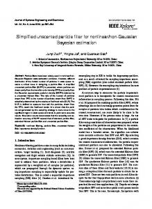
Figure 1: True trajectory of the single maneuvering target
IMM RPF PFPNI(Simplified) PFPNI(Complete)
45 40 35 RMSE in position (m)
where 𝑍𝑘 = [𝑧1 , 𝑧2 ]𝑘 is the observation vector. 𝑧1 is the distance between the radar and the target, and 𝑧2 is the bearing angle. The measurement noise 𝑛𝑘 = [𝑛𝑧1 , 𝑛𝑧2 ]𝑘 is a zero mean Gaussian white noise process with standard deviations of 20 𝑚 (𝜎𝑧1 ) and 0.01 𝑟𝑎𝑑 (𝜎𝑧2 ). Resolution of the sensor is selected after from [14] (twice of the standard deviations of the measurement noise). The sampling interval is Δ𝑇 = 1𝑠. The process noise identification based particle filter is compared to the IMM filter and the regularized particle filter. The IMM filter consists of three extended Kalman filter (EKF) with different motion models. The details regarding these models may be found in [13]. The initial model probabilities and the mode switching probability matrix are set the same values as in [13]. For the regularised particle filter, Epanechnikov kernel is chosen as the rescaled kernel density, which is same as in [15]. Moreover, the proposed algorithm is compared to its complete version in the same simulation setup. The simulation results are obtained from 1000 Monte Carlo runs. Fig. 1 shows the true trajectory of the maneuvering target. The root mean-square errors (RMSEs) in position at each time step respectively using the four methods are shown in Fig. 2, where RPF and PFPNI represent the regularised particle filter algorithm and the particle filter based process noise identification algorithm. The performance of the methods is also compared via the global RMSE (in position), the tracking loss rate (TLR) and the executing time (ET), which are listed in Table. 1. The tracking loss rate (TLR) is defined as the ratio of the number of simulations, in which the target is lost in track, to the total number of simulations carried out. The target is defined as lost in track when its global RMSE in position is larger than ten times of the magnitude of the standard deviation in position. The executing time (ET) is the CPU time needed to execute one time step in MATLAB 7.1 on a
30 25 20 15 10 5 0
0
20
40
60
80
100
Time (sec)
Figure 2: RMSE in position using IMM, RPF, PFPNI (simplified) and PFPNI (complete) algorithms
5
Conclusions
In this paper, a novel method, process noise identification based particle filter is proposed for tracking highly maneuvering target. The proposed method is based on the assumption that the random effect (including maneuvers and random noises) can be modeled by (part of) a white or colored noise process sufficiently
Table 1: Performance Comparison RMSE ET (s) TLR (m) IMM 28.34 0.0239 3.7% RPF 16.66 0.8708 0 PFPNI 0.4503 0 (simpli- 13.67 fied) PFPNI (com- 13.29 190.47 0 plete)
well. This fundamental assumption converts the problem of maneuvering target tracking to that of state estimation in presence of non-stationary process noise with unknown statistics. In order to identify the distribution of the process noise, the process noise is modeled as an individual dynamic system. A sampling based algorithm is then proposed in the particle filter framework to estimate the state vector (process noise) based on the current measurements. The predicted particles are then generated from the newly obtained process noise samples and are more close to the current state of the target, which can reduce the sample impoverishment effectively. The proposed algorithm is illustrated via an example involving tracking a highly maneuvering target.
References [1] A. H. Jazwinski, Stochastic processes and filtering theory. New York: Academic Press, 1970. [2] X. R. Li and Y. Bar-Shalom, “A recursive multiple model approach to noise identification,” IEEE Trans. Aerospace and Electronic Systems, vol. 30, no. 3, pp. 671–684, July 1994. [3] ——, “A recursive hybrid system approach to noise identification,” Proceedings of the first IEEE Conference on Control Applications, pp. 847–852, 1992. [4] R. Karlsson and F. Gustafsson, “Range estimation using angle-only target tracking with particle filters,” Proceedings of American Control Conference, vol. 5, pp. 3743–3748, 2001. [5] N. Ikoma, N. Ichimura, T. Higuchi, and H. Maeda, “Maneuvering target tracking by using particle filter,” IFSA World Congress and 20th NAFIPS International Conference, vol. 4, pp. 2223–2228, 2001. [6] R. Karlsson and N. Bergman, “Auxiliary particle filters for tracking a maneuvering target,” Proceedings of the 39th IEEE Conference on Decision and Control, vol. 4, pp. 3891–3895, 2000.
[7] N. Ikoma, T. Higuchi, and H. Maeda, “Tracking of maneuvering target by using switching structure and heavy-tailed distribution with particle filter method,” Proceedings of the 2002 International Conference on Control Applications, vol. 2, pp. 1282–1287, 2002. [8] W. Malcolm, A. Doucet, and S. Zollo, “Sequential Monte Carlo tracking schemes for maneuvering targets with passive ranging,” Proceedings of the Fifth International Conference on Information Fusion, vol. 1, pp. 482–488, 2002. [9] A. Doucet, J. F. G. de Freitas, and N. J. Gordon, Sequential Monte Carlo Methods in Practice. New York: Springer-Verlag, 2001. [10] M. Morelande and S. Challa, “Manoeuvring target tracking in clutter using particle filters,” IEEE Trans. Aerospace and Electronic Systems, vol. 41, no. 1, pp. 252–270, Jan. 2005. [11] S. J. Godsill, J. Vermaak, W. Ng, and J. F. Li, “Models and algorithms for tracking of maneuvering objects using variable rate particle filters,” Proceedings of the IEEE, vol. 95, no. 5, pp. 925– 952, May 2007. [12] M. Arulampalam, S. Maskell, N. Gordon, and T. Clapp, “A tutorial on particle filters for online nonlinear/non-Gaussian Bayesian tracking,” IEEE Transactions on Signal Processing, vol. 50 , pp. 174–188, 2002. [13] B. Chen and J. K. Tugnait, “Tracking of multiple maneuvering targets in clutter using IMM/JPDA filtering and fixed-lag smoothing,” Automatica, vol. 37, pp. 239–249, Feb. 2001. [14] W. Koch and G. Keuk, “Multiple hypothesis track maintenance with possibly unresolved measurements,” IEEE Transaction on Aerospace and Electronic Systems, vol. AES-33, pp. 883–892, 1997. [15] C. Musso, N. Oudjane, and F. LeGland, “Improving regularized particle filters,” in Sequential Monte Carlo Methods in Practice, A. Doucet, N. DeFreitas, and N. Gordon, Eds. New York: Springer, 2001, pp. 247–271.