Particle filtering based identification for autonomous nonlinear ODE

Particle filtering based identification for autonomous nonlinear ODE models ⋆ Jerker Nordh ∗ Torbj¨ orn Wigren ∗∗ Thomas B. Sch¨ on ∗∗ Bo Bernhardsson ∗ ∗

Department of Automatic Control, Lund University, SE-221 00 Lund, Sweden (e-mail: {jerker.nordh, bo.bernhardsson}@control.lth.se). ∗∗ Department of Information Technology, Uppsala University, SE-751 05, Uppsala, Sweden (e-mail: {torbjorn.wigren, thomas.schon}@it.uu.se.).

Abstract: This paper presents a new black-box algorithm for identification of a nonlinear autonomous system in stable periodic motion. The particle filtering based algorithm models the signal as the output of a continuous-time second order ordinary differential equation (ODE). The model is selected based on previous work which proves that a second order ODE is sufficient to model a wide class of nonlinear systems with periodic modes of motion, also systems that are described by higher order ODEs. Such systems are common in systems biology. The proposed algorithm is applied to data from the well-known Hodgkin-Huxley neuron model. This is a challenging problem since the Hodgkin-Huxley model is a fourth order model, but has a mode of oscillation in a second order subspace. The numerical experiments show that the proposed algorithm does indeed solve the problem. Keywords: Autonomous system, identification, neural dynamics, nonlinear systems, oscillation, particle filtering, periodic system, phase plane. 1. INTRODUCTION The identification of nonlinear autonomous systems is a fairly unexplored field. While a very large amount of work has been devoted to the analysis of autonomous systems, given an ordinary differential equation (ODE), the inverse problem has received much less attention. At the same time system identification based on particle filtering ideas is expanding rapidly. However, little attention has so far been given to identification of nonlinear autonomous systems. The present paper addresses this by presenting a new approach for identification of a nonlinear autonomous ODE model based on recently developed particle filtering methods. Furthermore, the paper presents new results on neural modeling, by applying the new algorithm to data generated by the well-known Hodgkin-Huxley model. These constitutes the two main contributions of the paper. As stated above, much work has been performed on the analysis of a given nonlinear autonomous system, see e.g. Khalil (1996). The classical analysis provided by e.g. Poincar´e provides tools for prediction of the existence of periodic orbits of a second order ODE. Bifurcation analysis and similar tools have also been widely applied to the analysis of chaos, common in nonlinear autonomous ODEs (Khalil, 1996; Li et al., 2007). There are much less publications on and connections to the inverse problem, i.e. the identification of an autonomous nonlinear ODE ⋆ This work was supported by the project Probabilistic modeling of dynamical systems (Contract number: 621-2013-5524) funded by the Swedish Research Council. (*) are members of the LCCC Linnaeus Center and the ELLIIT Excellence Center at Lund University.

from measured data alone. However, algorithms tailored for identification of second order ODEs from periodic data appeared in Wigren et al. (2003a), Manchester et al. (2011) and Wigren (2014). A result on identifiability that gives conditions for when a second order ODE is sufficient for modeling of periodic oscillations is also available, see Wigren and S¨ oderstr¨ om (2005) and Wigren (2015). That work proves that in case the phase plane of the data is such that the orbit does not intersect itself, then a second order ODE is always sufficient for identification. In other words, higher order models cannot be uniquely identifiable. There is a vast literature on stable oscillations in biological and chemical systems, see e.g. Rapp (1987). An important example is given by neuron spiking (Doi et al., 2002; Izhikevich, 2003; Hodgkin and Huxley, 1952). This spiking is fundamental in that it is the way nerve cells communicate, for example in the human brain. The field of reaction kinetics provides further examples of dynamic systems that are relevant in the field of molecular systems biology, see e.g. Ashmore (1975). Such kinematic equations typically result in systems of ordinary differential equations with right hand sides where fractions of polynomials in the states appear. The many authors that have dealt with identification of the Hodgkin-Huxley model have typically built on complete models, including an input signal current, see e.g. Doi et al. (2002); Saggar et al. (2007); Tobenkin et al. (2010); Manchester et al. (2011); Lankarany et al. (2013). With the exception of Wigren (2015) there does not seem to have been much work considering the fact that identification may not be possible if only periodic data is available.

The particle filter was introduced more that two decades ago as a solution to the nonlinear state estimation problem, see e.g. Doucet and Johansen (2011) for an introduction. However, when it comes to the nonlinear system identification problem in general, it is only relatively recently that the particle filter has emerged as a really useful tool, see Kantas et al. (2014) for a recent survey. The algorithm presented here is an adaptation of the so-called PSAEM algorithm introduced by Lindsten (2013). It provides a solution to the nonlinear maximum likelihood problem by combining the stochastic approximation expectation maximization algorithm of Delyon et al. (1999) with the PGAS kernel of Lindsten et al. (2014). This improves upon the earlier work of Wigren et al. (2003b), since it is no longer necessary to rely on the sub-optimal extended Kalman filter and restrictive models of the model parameters. 2. FORMULATING THE MODEL AND THE PROBLEM The periodic signal is modeled as the output of a second order differential equation, and can in continuous-time thus be represented as xt = (pt vt )T , (1a)   vt x˙ t = . (1b) f (pt , vt ) The discretized model is obtained by a Euler forward approximation and by introducing noise acting on the measurements and on the second state to describe the model errors pt+1 = pt + hvt , (2a) vt+1 = vt + hf (pt , vt ) + wt (2b) y t = pt + e t . (2c) The noise is only acting on one of the states, implying that one of the states can be marginalized. The previous choice of Euler forward gives a model where the required non-Markovian smoothing densities can be evaluated in constant time, for many formulations this does not hold and the time-complexity instead grows with the size of the dataset. The marginalization, which will prove useful later for the particle filter, results in the following nonMarkovian model pt+1 = pt + h(vt−1 + hf (pt−1 , vt−1 ) + wt−1 )   pt − pt−1 2 = 2pt − pt−1 + h f pt−1 , + h hwt−1 , (3a) y t = pt + e t , (3b) where the noise is assumed Gaussian according to wt−1 ∼ N (0, Qw ), et ∼ N (0, R). (3c) As suggested by Wigren et al. (2003b), the function f (p, v) is parametrized according to m X m X aij pi v j . (3d) f (p, v) = i=0 j=0

Here, m is a design parameter deciding the degree of the model used for the approximation and the indices aij denote unknown parameters to be estimated together with the process noise covariance Qw . Hence, the unknown parameters to be estimated are given by θ = {Qw a00 ... a0m ... am0 ... amm }. (4)

It has been assumed that the measurement noise covariance R is known. The problem under consideration is that of computing the maximum likelihood (ML) estimate of the unknown parameters θ by solving θbML = argmax log pθ (y1:T ), (5) θ

where y1:T = {y1 , . . . , yT } and pθ (y1:T ) denotes the likelihood function parameterized by θ. 3. PARTICLE FILTERING FOR AUTONOMOUS SYSTEM IDENTIFICATION

After the marginalization of the v state in model (2) the problem becomes non-Markovian, for an introduction to non-Markovian particle methods see e.g., Lindsten et al. (2014) and Lindsten and Sch¨ on (2013). The remainder of this section will go through the components required for the algorithm and note specific design choices made to apply the methods to the particular class of problems that are of interest in this paper. 3.1 Expectation maximization algorithms The expectation maximization (EM) algorithm (Dempster et al., 1977) is an iterative algorithm to compute ML estimates of unknown parameters (here θ) in probabilistic models involving latent variables (here, the state trajectory x1:T ). More specifically, the EM algorithm solves the ML problem (5) by iteratively computing the so-called intermediate quantity Z Q(θ, θk ) = log pθ (x1:T , y1:T )pθk (x1:T | y1:T )dx1:T (6) and then maximizing Q(θ, θk ) w.r.t. θ. There is now a good understanding of how to make use of EM-type algorithms to identify dynamical systems. The linear state space model allows us to express everything in closed form (Shumway and Stoffer, 1982; Gibson and Ninness, 2005). However, when it comes to nonlinear models, like the ones considered here, approximate methods have to be used, see e.g. (Lindsten, 2013; Sch¨ on et al., 2011; Capp´e et al., 2005). The sequential Monte Carlo (SMC) methods (Doucet and Johansen, 2011) or the particle Markov chain Monte Carlo (PMCMC) methods introduced by Andrieu et al. (2010) can be exploited to approximate the joint smoothing density (JSD) arbitrarily well according to N X wTi δxi1:T (x1:T ). (7) pb(x1:T | y1:T ) = i=1

Here, xi1:T denotes the i:th sample of x1:T , the notation x1:T is used for the collection (x1 , ..., xT ). wTi denotes the weights given to the i:th sample and δx denotes a pointmass distribution at x. Sch¨ on et al. (2011) used the SMC approximation (7) to approximate the intermediate quantity (6). However, there is room to make even more efficient use of the particles in performing ML identification, by making use of the stochastic approximation developments within EM according to Delyon et al. (1999). In the socalled stochastic approximation expectation maximization (SAEM) algorithm, the intermediate quantity (6) is replaced by the following stochastic approximation update bk (θ) = (1 − γk )Q bk−1 (θ) + γk log pθ (x1:T [k], y1:T ), (8) Q

where γk denotes the step design paP∞size, which is a P ∞ rameter that must fulfill k=1 γk = ∞ and k=1 γk2 < ∞. Furthermore, x1:T [k] denotes a sample from the JSD pθk (x1:T | y1:T ). The sequence θk generated by the SAEM algorithm outlined above will under fairly weak assumptions converge to a maximizer of pθ (y1:T ) (Delyon et al., 1999). For the problem under consideration the recently developed PMCMC methods (Andrieu et al., 2010; Lindsten et al., 2014) are useful to approximately generate samples from the JSD. This was realized by Lindsten (2013), resulting in the so-called particle SAEM (PSAEM) algorithm, which is used in this work.

system {xi1:T , wTi }N i=1 that is then used to approximate the intermediate quantity according to N X bk (θ) = (1 − γk )Q bk−1 (θ) + γk Q wTi log pθ (xi1:T , y1:T ). i=1

(11) Note that similarly to (8) only the reference trajectory x1:T [k] could have been used, but in making use of the entire particle system the variance of the resulting state estimates are reduced (Lindsten, 2013). The result is provided in Algorithm 2. Algorithm 2 PSAEM for sys. id. of autonomous systems 1: Initialization: Set θ[0] = (Qw 0

3.2 The PGAS kernel The particle Gibbs with ancestor sampling (PGAS) kernel was introduced by Lindsten et al. (2014). It is a procedure very similar to the standard particle filter, save for the fact that conditioning on one so-called reference trajectory x′1:T is performed. Hence, x′1:T have to be retained throughout the sampling procedure. For a detailed derivation see Lindsten et al. (2014), where it is also shown that the PGAS kernel implicitly defined via Algorithm 1 is uniformly ergodic. Importantly, it also leaves the target density p(x1:T | y1:T ) invariant for any finite number of particles N > 1 implying that the resulting state trajectory x⋆1:T can be used as a sample from the JSD. The notation used in Algorithm 1 is as follows, xt = (x1t , . . . , xN t ) denotes all the particles at time t and x1:T = (x1 , . . . , xT ) the entire trajectories. The particles are propagated according to a proposal distribution rt (xt | xt−1 , yt ). The resampling step and the propagation step of the standard particle filter has been collapsed into jointly sampling the particles {xit }N i=1 and the ancestor indices {ait }N i=1 independently from w at t Mt (at , xt ) = PN t rt (xt | xa1:t−1 , y1:t ). (9) l w l=1 t Finally, Wt denotes the weight function, p(yt | x1:t )p(xt | x1:t−1 ) . (10) Wt (x1:t , y1:t ) = r(xt | x1:t−1 , y1:t ) Algorithm 1 PGAS kernel 1: Initialization (t = 1): Draw xi1 ∼ r1 (x1 |y1 ) for i = 1, . . . , N − ′ i i 1 and set xN 1 = x1 . Compute w1 = W1 (x1 ) for i = 1, . . . , N . 2: for t = 2 to T do 3: Draw {ait , xit } ∼ Mt (at , xt ) for i = 1, . . . , N − 1. ′ 4: Set xN t = xt . 5:




N Draw aN t with P at = i ∝ ai

wi

5: 6: 7: 8: 9: 10: 11: 12: 13:

FFBSi particle smoother. Set = 0 and set w[0] to an empty vector. Draw x′1:T using FFBSi. for k ≥ 1 do Draw x1:T [k], wT by running Algorithm 1 using x′1:T as reference. i . Draw j with P (j = i) = wT Set x′1:T = xj1:T [k] Set w[k] = ((1 − γk )w[k − 1] γk wT ) bk (θ) according to (11). Compute Q bk (θ). Compute θ[k] = argmax Q if termination criterion is met then return {θ[k]} end if end for

Note that the initial reference trajectory x1:T [0] is obtained by running a so-called forward filter backward simulator (FFBSi) particle smoother, see Lindsten and Sch¨ on (2013) for details. To indicate that the trajectories were generated at iteration k, we use x1:T [k] and analogously for the weights. The 9th row of Algorithm 2 will for the model (3) under consideration amount to a weighted least squares problem, which is solved in Algorithm 3. For the work presented in this article the termination criterion of Algorithm 2 is chosen as a fixed number of iterations. Algorithm 3 Maximizing Q 1: For each trajectory in x1:T [k] calculate the velocity at each time (i) (i) (i) vt = (pt+1 − pt )/h 2: For each time step and for each trajectory in x1:T [k], evaluate (i) (i) f (pt , vt ). 3: Find a00 ...amm via the related weighted least squares (WLS) problem. 4: Find Qw by estimating the covariance of the residuals of the WLS-problem. 5: Set θ[k] = {Qw a00 ... amm }.

p(x′t | xi1:t−1 )

PN t−1l l=1

2: 3: 4:

0T ) and set x1:T [0] using an

b0 Q

wt−1 p(x′t | xl1:t−1 )

t 6: Set xi1:t = {x1:t−1 , xit } for i = 1, . . . , N . i 7: Compute wt = Wt (xi1:t , y1:t ) for i = 1, . . . , N . 8: end for 9: Return x1:T , wT .

3.3 Identifying autonomous systems using PSAEM The PSAEM algorithm for ML identification of autonomous systems now simply amounts to making use of the PGAS kernel in Algorithm 1 to generate a particle

3.4 Choosing the proposal distribution The proposal density r(xt |x1:t−1 , y1:t ) constitutes an important design choice of the particle filter that will significantly affect its performance. The commonly used bootstrap particle filter amounts to making use of the dynamics to propose new particles, i.e. r(xt |x1:t−1 , y1:t ) = p(xt | x1:t−1 ). However, we will make use of the measurement model and the information present in the current measurement to propose new particles, i.e. r(xt |x1:t−1 , y1:t ) = p(yt | xt ). This is enabled by the marginalization of the deterministic state in the model, since the dimension of

2.5 2 Parameter value

the state-space then matches that of the measurement. As a possible further improvement, the proposal could also include the predicted state using the model. Recently, Kronander and Sch¨ on (2014) showed that the combined use of both the dynamics and the measurements results in competitive algorithms. In such a scenario the estimated uncertainty in the model would initially be large and thus not affect the proposal distribution significantly, but for each iteration of the PSAEM algorithm the model will be more and more accurate in predicting the future states, and its influence on the proposal distribution would increase accordingly.

1.5 1 0.5 0

−0.5 −1 −1.5

4. NUMERICAL ILLUSTRATIONS The performance of the proposed algorithm is illustrated using two examples, namely the Van der Pol oscillator in Section 4.1 and the Hodgkin-Huxley neuron model in Section 4.2 – 4.3. There is no prior knowledge of the model, hence it is assumed that all the parameters aij in (3d) are zero. The initial covariance Qw 0 is set to a large value. The Python source code for the following examples can be downloaded from Nordh (2015a), the implementation was carried out using the pyParticleEst software framework (Nordh, 2015b, 2013).

−2 −2.5 −3 0

5

10

15

20 25 30 iteration

35

40

45

50

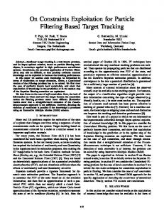
Fig. 1. Parameter convergence for the Van der Pol example (12). The dashed lines are the coefficients obtained from the discretization of the model, the other lines represent the different parameters in the identified model. Note that while the parameters do not converge to the ’true’ values, they provide a very accurate model for predicting the signal as shown in Fig. 3.

4.1 Validation on the Van der Pol oscillator

T

where xt = (pt vt ) . Performing 50 iterations of Algorithm 2 gives the parameter convergence shown in Fig. 1. Here N = 15 particles were used for the PGAS sampler, and the model order was chosen as m = 2. The dataset was sampled with h = 0.025s. For the SAEM step, the sequence γ1:K is chosen as  1 if k ≤ 5, γk = (13) (k − 5)−0.9 if k > 5. It can be seen that the parameters converge to values close to those obtained from the Euler forward discretization. To analyze the behavior further the phase-plane for the system is shown in Fig. 2 and the time-domain realization in Fig. 3. Here it can be seen that the identified model captures the behavior of the true continuous-time system significantly better than the model obtained from the discretization. 4.2 The Hodgkin-Huxley neuron model The well-known Hodgkin-Huxley model uses a nonlinear ODE to describe the dynamics of the action potentials in a neuron. In this paper the model will be used for two purposes. First, simulated spiking neuron data is used to characterize the performance of the proposed algorithm when identifying a nonlinear autonomous system. It should be noted that the data does not correspond to a system that is in the model set. The ability to handle nonlinear

3 2 1 v

To demonstrate the validity of the proposed solution it is first applied to the classic Van der Pol oscillator (Khalil, 1996), which belongs to the model class defined by (3). The oscillator is described by   vt , (12) x˙ t = −pt + 2(1 − p2t )vt

True Predicted Measurements

4

0

−1 −2 −3 −4 −2 −1.5

−1 −0.5

0 p

0.5

1

1.5

2

Fig. 2. Phase-plane plot for the Van der Pol example (12). under-modeling is therefore also assessed. Secondly, the new algorithm and the identification results contribute to an enhanced understanding of spiking neurons by providing better performance compared to previous algorithms. The Hodgkin-Huxley model formulation of Siciliano (2012) is used, where the following ODE is given dv 1  = I − gna m3 h(v − Ena ) dt Cm  ×gK n4 (v − EK ) − gl (v − El ) , dn = αn (v)(1 − n) − βn (v)n, dt dm = αm (v)(1 − m) − βm (v)m, dt dh = αh (v)(1 − h) − βh (v)h. dt

(14a) (14b) (14c) (14d)

2.5

True Predicted Discretized

2 1.5 1

p

0.5 0

Fig. 5 shows the same dataset in the time-domain, it shows the true signal (without added noise) and the output predicted by the identified model when initialized with the correct initial state. It can be seen that the model captures the behaviour of the signal, but introduces a small error in the frequency of the signal, causing the predicted and true signal to diverge over time. 350

−0.5

True Predicted Measurements

300

−1 250

−1.5

200

−2.5 0

200

400

600

800 1000 1200 1400 1600 1800 2000 t

Fig. 3. Predicted output using the true initial state and the estimated parameters. The plot labeled ”discretized” is obtained by discretization of the true continuoustime model using Euler forward and using that to predict the future output. It can been seen that the discretized model diverges over time from the true signal, clearly the identified parameter values give a better estimate than using the values from the discretization. Here, v denotes the potential, while n, m and h relate to each type of gate of the model and their probabilities of being open, see Siciliano (2012) for details. The applied current is denoted by I. The six rate variables are described by the following nonlinear functions of v

αh (v) = 0.07e

−0.05(v+60)

,

50 0 −50 −60

−40

−20

p

0

20

40

60

Fig. 4. Phase-plane for the Hodgkin-Huxley dataset. It can be seen that the predicted model fails to capture the initial transient, but accurately captures the limit cycle. 60

(15a)

40

(15b)

20

(15c)

0

(15d) (15e)

1

. (15f) 1+ The corresponding numerical values are given by Cm = 0.01 µF/cm2 , gN a = 1.2 mS/cm2 , EN a = 55.17 mV , gK = 0.36 mS/cm2 , EK = −72.14 mV , gl = 0.003 mS/cm2 , and El = −49.42 mV . βh (v) =

100

True Predicted

p

0.01(v + 50) , 1 − e−(v+50)/10 βn (v) = 0.125e−(v+60)/80, 0.1(v + 35) , αm (v) = 1 − e−(v+35)/10 βm (v) = 4.0e−0.0556(v+60) , αn (v) =

150 v

−2

−20 −40

e−0.1(v+30)

4.3 Identifying the spiking mode of the Hodgkin-Huxley model Using a simulated dataset of length T = 10 000 sampled with h = 0.04s, a model of the form (3) with m = 3 is selected. Algorithm 2 was run for 200 iterations, employing N = 20 particles in the PGAS kernel. For the SAEM step, the sequence γ1:K is chosen as  1 if k ≤ 40, γk = (16) (k − 40)−0.5 if k > 40. The predicted phase-plane of the identified model is shown in Fig. 4 along with the true phase-plane and the measurements.

−60 −80 0

1000 2000 3000 4000 5000 6000 7000 8000 9000 10000 t

Fig. 5. Predicted output using the true initial state and the estimated parameters. The overall behaviour of the signal is captured, but there is a small frequency error which leads to the predicted signal slowly diverging from the true signal. 5. CONCLUSIONS The new identification method successfully identified models for both the Van der Pol example and for the more complex Hodgkin-Huxley model. Even though the HodgkinHuxley model in general cannot be reduced to a second order differential equation it is possible to identify a good second order model for its limit cycle as shown in Fig. 4.

The use of a Bayesian nonparametric model in place of (3d) constitutes an interesting continuation of this work. A first step in this direction would be to employ the Gaussian process construction by Frigola et al. (2013, 2014). Another interesting topic for future research is the question of asymptotic stability of the periodic solutions of the estimated models. Based on the selected model structure, this problem could be approached with standard tools from nonlinear systems theory, including invariant sets and Poincar´e maps, see (Khalil, 1996, chapter 7.3). Furthermore the authors see no reason that the method could not be extended to identify the noise covariance as well, but for the work done here it was left as a design variable. REFERENCES Andrieu, C., Doucet, A., and Holenstein, R. (2010). Particle Markov chain Monte Carlo methods. Journal of the Royal Statistical Society, Series B, 72(2), 1–33. Ashmore, P.G. (1975). Kinetics of Oscillatory Reactions. The Chemical Society. Capp´ e, O., Moulines, E., and Ryd´ en, T. (2005). Inference in Hidden Markov Models. Springer Series in Statistics. Springer, New York, USA. Delyon, B., Lavielle, M., and Moulines, E. (1999). Convergence of a stochastic approximation version of the EM algorithm. The Annals of Statistics, 27(1), 94–128. Dempster, A.P., Laird, N.M., and Rubin, D.B. (1977). Maximum likelihood from incomplete data via the EM algorithm. Journal of the Royal Statistical Society B, 39(1), 1–38. Doi, S., Onada, Y., and Kumagai, S. (2002). Parameter estimation of various Hodgkin-Huxley-type neuronal models using a gradientdescent learning method. In Proceedings of the 41st SICE Annual Conference, 1685–1688. Osaka, Japan. Doucet, A. and Johansen, A.M. (2011). A tutorial on particle filtering and smoothing: Fifteen years later. In D. Crisan and B. Rozovsky (eds.), Nonlinear Filtering Handbook. Oxford University Press. Frigola, R., Lindsten, F., Sch¨ on, T.B., and Rasmussen, C.E. (2013). Bayesian inference and learning in Gaussian process state-space models with particle MCMC. In Advances in Neural Information Processing Systems (NIPS) 26, 3156–3164. Frigola, R., Lindsten, F., Sch¨ on, T.B., and Rasmussen, C.E. (2014). Identification of Gaussian process state-space models with particle stochastic approximation EM. In Proceedings of the 18th World Congress of the International Federation of Automatic Control (IFAC). Cape Town, South Africa. Gibson, S. and Ninness, B. (2005). Robust maximum-likelihood estimation of multivariable dynamic systems. Automatica, 41(10), 1667–1682. Hodgkin, A.L. and Huxley, A.F. (1952). A quantitative description of membrane current and its application to conduction and excitation in nerve. The Journal of Physiology, 117(4), 500–544. Izhikevich, E.M. (2003). Simple models of spiking neurons. IEEE Transactions on Neural Networks, 14(6), 1569–1572. Kantas, N., Doucet, A., Singh, S.S., Maciejowski, J., and Chopin, N. (2014). On particle methods for parameter estimation in statespace models. ArXiv:1412.8695, submitted to Statistical Science. Khalil, H.K. (1996). Nonlinear Systems. Prentice Hall, Upper Saddle River. Kronander, J. and Sch¨ on, T.B. (2014). Robust auxiliary particle filters using multiple importance sampling. In Proceedings of the IEEE Statistical Signal Processing Workshop (SSP). Gold Coast, Australia. Lankarany, M., Zhu, W.P., and Swamy, N.S. (2013). Parameter estimation of Hodgkin-Huxley neuronal model using dual extended Kalman filter. In Proceedings of the IEEE International Sym-

posium on Circuits and Systems (ISCAS), 2493–2496. Beijing, China. Li, H.Y., Che, Y.Q., Gao, H.Q., Dong, F., and Wang, J. (2007). Bifurcation analysis of the Hodgkin-Huxley model exposed to external DC electric field. In Proceedings of the 22nd International Symposium on Intelligent Control (ISIC), 271–276. Singapore. Lindsten, F. (2013). An efficient stochastic approximation EM algorithm using conditional particle filters. In Proceedings of the 38th International Conference on Acoustics, Speech, and Signal Processing (ICASSP). Vancouver, Canada. Lindsten, F., Jordan, M.I., and Sch¨ on, T.B. (2014). Particle Gibbs with ancestor sampling. Journal of Machine Learning Research (JMLR), 15, 2145–2184. Lindsten, F. and Sch¨ on, T.B. (2013). Backward simulation methods for Monte Carlo statistical inference. Foundations and Trends in Machine Learning, 6(1), 1–143. Manchester, I., Tobenkin, M.M., and Wang, J. (2011). Identification of nonlinear systems with stable oscillations. In Proceedings of the 50th IEEE Conference on Decision and Control and European Control Conference (CDC-ECC), 5792–5797. Orlando, FL, USA. Nordh, J. (2013). pyParticleEst software framework. URL http://www.control.lth.se/Staff/JerkerNordh/ pyparticleest.html. Nordh, J. (2015a). Example source code for ”Particle filtering based identification for autonomous nonlinear ode models”. URL http://www.control.lth.se/Staff/JerkerNordh/ode-id.html. Nordh, J. (2015b). pyParticleEst: A Python framework for particle based estimation methods. Journal of Statistical Software. Provisionally accepted. Rapp, P. (1987). Why are so many biological systems periodic? Progress in Neurobiology, 29(3), 261–273. Saggar, M., Mericli, T., Andoni, S., and Miikulainen, R. (2007). System identification for the Hodgkin-Huxley model using artificial neural networks. In Proceedings of the International Joint Conference on Neural Networks. Orlando, FL, USA. Sch¨ on, T.B., Wills, A., and Ninness, B. (2011). System identification of nonlinear state-space models. Automatica, 47(1), 39–49. Shumway, R.H. and Stoffer, D.S. (1982). An approach to time series smoothing and forecasting using the EM algorithm. Journal of Time Series Analysis, 3(4), 253–264. Siciliano, R. (2012). The Hodgkin–Huxley model – its extensions, analysis and numerics. Technical report, Department of Mathematics and Statistics, McGill University, Montreal, Canada. Tobenkin, M.M., Manchester, I., Wang, J., Megretski, A., and Tedrake, R. (2010). Convex optimization in identification of stable non-linear state space models. In Proceedings of the 49th IEEE Conference on Decision and Control (CDC), 7232–7237. Atlanta, USA. Wigren, T. (2014). Software for recursive identification of second order autonomous systems. Technical report, Department of Information Technologt, Uppsala University, Uppsala, Sweden. URL http://www.it.uu.se/research/publications/ reports/2014-014/SWAutonomous.zip. Wigren, T. (2015). Model order and identifiability of non-linear biological systems in stable oscillation. IEEE/ACM Transactions on Computational Biology and Bioinformatics. Accepted for publication. Wigren, T., Abd-Elrady, E., and S¨ oderstr¨ om, T. (2003a). Harmonic signal analysis with Kalman filters using periodic orbits of nonlinear ODEs. In Proceedings of the IEEE International Conference on Acoustics, Speech, and Signal Processing (ICASSP), 669–672. Hong Kong, PRC. Wigren, T. and S¨ oderstr¨ om, T. (2005). A second order ODE is sufficient for modeling of many periodic systems. International Journal of Control, 77(13), 982–986. Wigren, T., Abd-Elrady, E., and S¨ oderstr¨ om, T. (2003b). Least squares harmonic signal analysis using periodic orbits of ODEs. In Proceeding of 13th IFAC symposium on system identification (SYSID), 1584–1589. Rotterdam, The Netherlands.