Particle image velocimetry in a variable density flow - Springer Link

Experiments in Fluids 17 (1994)434-440 © SpringerVerlag 1994

Particle image velocimetry in a variable density flow: application to a dynamically evolving microburst A. Alahyari, E. K° Longmire

434

Abstract A fundamental difficulty in the experimental study of gravity-driven flows using particle image velocimetry (PIV) and other optical diagnostic techniques is the problem associated with variations in the refractive index within the fluid. This paper discusses a method by which the refractive indices of two fluids are matched while maintaining density differences of up to 4%- Aqueous solutions of glycerol and potassium phosphate are used to achieve precise index matching in the presence of mixed and unmixed constituents. The effectiveness of the method is verified in a PIV study of a laboratory-scale model of an atmospheric microburst where planes of two-dimensional velocity vectors are obtained in the evoiving flow field. 1 Introduction In gravity-driven or other variable density flows, the index of refraction changes with the local value of the density. It is well known that variations in the refractive index within a flow cause problems with the application of laser Doppler velocimetry (LDV). The laser beams bend as they pass through fluid of varying refractive index. Hence, the location of the measuring volume changes with time, resulting in decreased data detection rates. Furthermore, Doppler frequencies detected from seed particles traversing the measuring volume can be shifted due to laser beam motion, resulting in systematic errors and "artificial turbulence". Particle image velocimetry suffers from similar undesirable effects. Application of PIV involves seeding the flow with small reflective particles and illuminating a slice of the flow field with a thin sheet of pulsed laser light. Photographs of light scattered from the sheet are taken using a 35 mm camera where the film is exposed long enough to capture two laser pulses. An ideal photograph for PIV analysis contains two distinct images for every particle within the light sheet. However, when light scattered from seed particles travels through a region of non-uniform refractive index, it bends in different directions depending on the local refractive index

Received: 11 November 1993/Accepted: 7 June 1994

A. Alahyari, E. K. Longmire Department of Aerospace Engineering and Mechanics, University of Minnesota, Minneapolis, MN 55455 USA Correspondence to: A. Alahyari

This work was sponsored by the National Science Foundation under grant CTS-9zo9948. We also thank TSI, Inc. for the use of its facility

and on the angle it makes with the interface between the two fluids. This can result in a blurred image on the film where individual particle images cannot be distinguished. The severity of this effect also depends on the distance the light must travel through this region. The longer the distance, the greater the potential problem. One way of avoiding this problem is to ensure a uniform refractive index throughout the flow. McDougall (1979) developed a method of matching the refractive indices of two fluids while maintaining a density difference. He used sugar and Epsom salt as solutes in water to produce two appropriate fluids. Hannoun et al. (1988) used ethyl alcohol and salt (NaC1) as the two solutes to achieve the same effect. Hence, the idea of matching refractive indices of two fluids is not new, but questions remain regarding practicality, cost, and the material properties of the resulting solutions. In this study, a new pair of solutes, glycerol and potassium dihydrogen phosphate (monobasic), was found to be an appropriate choice for PIV studies on model downbursts. In several ways, this combination proves superior to the combinations used in previous studies. The process of matching the refractive index and the significant factors that need to be considered are discussed in Sect. 2. The index matching strategy was applied in a flow of a simulated microburst. An atmospheric microburst (downburst) is a small, localized flow of relatively heavy cold air which rushes downward and spreads radially outward as it nears the ground. The downflow shaft is often encircled by a horizontal vortex ring which is responsible for intense outward winds. Although this phenomenon is short-lived, lasting only five to ten minutes, it can generate extreme windshears (sudden variations in wind velocity) which pose a significant threat to aircraft. Thus, a greater understanding of the behavior of microbursts is needed to provide safer travel for aircraft that encounter these structures. The most direct method of investigating atmospheric microbursts is through field experiments. However, since microbursts occur rapidly and are difficult to forecast, obtaining data on actual microbursts has been difficult and expensive. Northern Illinois Meteorological Research on Downbursts (NIMROD) 1978 and ]oint Airport Weather Studies (]AWS) 1982 were two major field experiments in the United States conducted to investigate microbursts (Fujita 1985). These studies provided information so appropriate length and time-scales for the 'average' microburst could be established, and as a result, model studies could be related to full-scale atmospheric microbursts. The field studies revealed only a weak correlation between microburst occurrences and the local meteorological conditions

such as temperature, pressure or humidity. Thus, prediction of microbursts based purely on ambient environmental conditions did not seem promising. Large-scale numerical models based on large-eddy-simulation (LES) methods have provided a significant amount of information on the structure of microbursts (Proctor 1987, Droegemeier 1988) but they require broad assumptions concerning the initial and boundary conditions. Hence, it is not known whether these studies have modeled the near-ground behavior of microbursts correctly. (This is also the region where Doppler radar measurements of actual microbursts are the most incomplete.) Flow visualization and some quantitative experiments have been conducted on small-scale simulated microbursts (Fujita 1986, Lundgren et al. 1992). Lundgren et al. (1992) developed and validated an important scaling law to relate the simulated structures to much larger atmospheric microbursts. Due to the complexity and transient nature of the simulated flow, conventional methods for velocity measurement are either inappropriate or difficult to implement. These methods involve the use of hot films or laser Doppler velocimeters. There are several problems associated with applying these techniques to reconstruct the entire velocity field. First, the presence of velocity probes such as hot films can seriously disturb the flow. Second, the use of hot-film probes in highly turbulent or reversing flow fields results in large errors. Third, since these techniques involve single point measurements, a twodimensional velocity field can be reconstructed only through a long series of sequential measurements. Although this procedure can be applied to steady flows rather easily, it is impractical for investigating an unsteady downburst flow. Also, refractive index fluctuations have been a major obstacle to the study of this type of flow using either LDV or the newer technique of PIV. It is believed that the current experiments demonstrate the first successful application of PIV in a variable density flow. The experimental facility, application of PIV, and the significant parameters are discussed in Section 3. 2

Matching the refractive index The procedure adopted here involves using a solution of glycerol and water as the less dense tank fluid and an aqueous solution of potassium dihydrogen phosphate as the heavier downburst fluid. Table 1 shows that, for instance, a 6% solution of glycerol and a 6% solution of potassium phosphate have the same refractive index but a 3% density difference. A Reichert 10419 hand-held refractometer is used to match the refractive indices to within o.oool. In the current experiments, glycerol has certain advantages over sugar used by McDougall and ethyl alcohol used by Hannoun. A sugar solution carries a relatively high cost, is difficult to handle and clean up, and attracts insects and microorganisms. Ethyl alcohol has other disadvantages; for example, due to its high volatility, it is difficult to use in facilities where large free surfaces exist. Glycerol is a clear, odorless liquid that is miscible in water and does not evaporate or react with the environment. It is easy to handle and remains transparent when left in a large tank for up to ten days. Potassium phosphate (KH2PO4) was chosen for the heavier solution since for a solution of fixed density, it increases the index of refraction less than most other salts. Therefore, a lower concentration of glycerol is required to match the refract-

ive index. Potassium phosphate, while not as common as table salt, is typically less expensive than Epsom salt. The chosen solute pair provides solutions that satisfy several other criteria important for the flow considered. First, up to a significant density difference, the index of refraction remains uniform when the two fluids are mixed. In general, the nonlinearity of the index of refraction as a function of solute concentration can result in variations in the index when mixing occurs. This property of the index of refraction creates an upper limit for the density difference that can be obtained, which in turn, for a given facility, imposes a limit on the maximum achievable Grashof or Reynolds number. The maximum allowable variation in the index of refraction, (An) . . . . is a function of the measurement technique as well as the distance the light must travel through the region of varying refractive index. It appears that for a fixed upper limit on An, glycerol and potassium phosphate solutions can provide a larger density difference than either sugar and Epsom salt or ethyl alcohol and table salt. Experiments show that a 4% density difference can be achieved with a maximum An of o.oool. This value of An was given by Hannoun (1985) as the maximum allowable change in the refractive index for LDV applications where the beams traverse a distance of 30 cm through the liquid mixture. Results from the present study indicate that PIV images are also extremely intolerant to small index variations. Variations in the index as small as 0.0002 are sufficient to render our PIV pictures unusable. The chosen pair of solutions does not yield double diffusive convection at the interface between the two fluids. This was tested by visualizing a layer of glycerol in water lying above a potassium phosphate solution. A small amount of dye was Table. 1. Chemicalproperties of glycerol and potassium phosphate(monobasic) in aqueous solutions. (Table from CRCHandbookof Chemistry and Physics) % by wt.

SG

n

#1#o

Glycerol 0.5 1 2 3 4 5 6 7 8 9 10

1.0011 1.0023 1.0046 1.0069 1.0092 1.0115 1.0138 1.0162 1.0185 1.0209 1.0233

1.3336 1.3342 1.3353 1.3365 1.3376 1.3388 1.34 1.3412 1.3424 1.3436 1.3448

1.009 1.02 1.046 1.072 1.098 1.125 1.155 1.186 1.218 1.253 1.288

Potassium phosphate 0.5 1.0035 1 1.0071 2 1.0143 3 1.0215 4 1.0288 5 1.036 6 1.0432 7 1.0505 8 1.0577 9 1.0649 10 1,0722

1.3336 1.3342 1.3354 1.3365 1.3377 1.3388 1.34 1.3411 1.3422 1.3434 1.3445

1.008 1.017 1.036 1.058 1.081 1.106 1.131 1.158 1.185 1.213 1.243

435

436

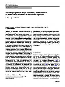
added to the glycerol solution, and the interface was observed for a period of 6o minutes. No evidence of motion other than diffusive thickening of the interface was observed. Finally, the glycerol-potassium phosphate combination yields two fluids with a small difference in viscosity. For solutions with a 3% density difference, this pair of solutes yields a difference in viscosity of only 2% compared with a difference of about 30% for a similar index-matched combination of ethyl alcohol and salt solutions (see Table 1). This is mainly because at typical concentrations in aqueous solutions (up to 30% by weight), glycerol increases viscosity less than ethyl alcohol (see Fig. 1). Variations in viscosity, while often neglected, create difficulty in determining the true Reynolds number or Grashof number of the flow. Also, in the context of atmospheric downbursts, the typical viscosity difference between the colder inner and warmer outer fluids is on the order of 2-3%.

ts. /

glycerol

1.4tso ~t ~2 1~ 1.0 percent by

weight

Fig. 1. Relative viscosities of glycerol and ethyl alcohol vs. solute concentration. (From CRC Handbook of Chemistry and Physics)

3

Experimental verification using PIV In this study, a downburst is modeled by releasing a small volume of heavier fluid into a tank containing a less dense fluid. The downburst fluid impinges on a horizontal circular plate which represents the ground. The impingement of the heavier fluid onto the flat surface produces a transient stagnation point flow. The flow is dominated by a turbulent vortex ring that develops through baroclinic generation of vorticity. Countervorticity (vorticity with opposite circulation) is generated due to friction along the boundary layer that forms on the horizontal surface. Lundgren et al. (1992) developed an important scaling law to relate the simulated microbursts to large-scale atmospheric microbursts. The corresponding mathematical model neglects diffusion between the lighter and heavier fluids, and assumes inviscid and incompressible flow. Also, the density difference, Ap, between the two fluids is assumed to be small enough that the Boussinesq approximation holds. The time scale of the flow is defined as

_ f Rop ~ ~/2

To- ~g~p)

'

(3.1)

where Ro is the spherical radius of the downburst parcel (spherical radius is defined as the radius of a sphere having the same volume). A Reynolds number is then defined as

VoRo

Re = - - ,-p

(3.z)

where Vo=Ro/To is the velocity scale. Lundgren et al. (1992) showed that microburst evolution is independent of Reynolds number when the Reynolds number is larger than 300o. Therefore, despite the fact that this gravity-driven flow lacks some of the meteorological features associated with real microbursts, we believe that at sufficiently large Reynolds numbers, it displays the main characteristics of the large scale structure. ].1

Flow facility The flow is contained in a large glass tank with inner dimensions of 76o mm × 760 mm x 915 mm. In order to minimize wall

solenoid

q D-610mm

Fig. 2. Flow modeling facility

effects, the downburst fluid impinges on a horizontal, circular plate of 61o mm diameter positioned 45o mm above the bottom of the tank. Figure 2 shows the flow modeling facility. The downburst release mechanism consists of a cylindrical container and a solenoid which drives a piercing needle. The cylinder has an inside diameter of 63.5 mm and a height of 87.0 mm. The total volume of the cylinder is 244 cm 3, and its spherical radius is 38.8 mm. The cylinder is open at the bottom and contains holes drilled at the top to a porosity of 50%. A thin latex sheet is stretched over the bottom of the cylinder which is then filled with the heavier downburst fluid. At the time of release, the piercing needle travels approximately i cm and bursts the latex sheet. The needle speed is kept low by reducing the voltage input to the solenoid as far as possible without loss of repeatability. This minimizes disturbances caused by the exploding latex sheet. Also, to make the retaining membrane more brittle, the latex sheet is aged in an oven before use.

3.2 Flow diagnostic Figure 3 shows a schematic of the PIV system used for investigating this flow. The flow field is illuminated by two frequency-doubled Surelite I Nd: YAG lasers which emit light at 532 nm. The lasers pulse at a frequency of lO Hz with a pulse duration of 7 ns and a maximum output energy of approximately 20o m] per pulse. The lasers are triggered externally during the experiment to achieve a rapid sequence of two pulses with controllable separation. The laser beams are converted into a thin (1 ram) sheet of light by using a i m focal length spherical lens and a 19 mm focal length cylindrical lens. The flow is seeded with Ti02 particles with a specific gravity of 3.5 and nominal diameter of 3 ~tm. The inertial time constant for these particles is on the order of I microsecond. The terminal velocity of the particles due to gravity is approximately 12 y/m/s, which is much smaller than typical velocities measured within the flow. Therefore, it is expected that these particles are capable of tracking all scales of the fluid motion. A Nikon NSoo8s 35 mm camera and a Nikon AF Micro-Nikkor lens with focal length of lo5 mm are used to photograph the flow field. The camera has a vertical-travel shutter which can be triggered electronically. Photographs of the illuminated flow field are recorded on Technical Pan black and white film using an aperture of f/4 and an image magnification M of o.16o +_ o.ool. The camera shutter speed is set to 67 ms so only one pair of pulses is captured on the film. To resolve directional ambiguity in the velocity field, a method known as spatial image shifting, proposed by Adrian (1986), is employed. This method involves shifting the entire image field by a known distance which is larger than and opposite to that caused by the maximum negative velocity in a certain direction. As a result, the largest negative velocity vector still yields a positive image shift. After interrogation of the film, the imposed shift is subtracted to determine the actual velocity. Image shifting is achieved by placing a rotating mirror assembly in front of the photographing lens. The flat mirror has dimensions of 44 mm × 54 mm and is mounted with its axis of rotation parallel to the longer dimension yielding a mass moment of inertia of 3o g-cm 2 about the rotation axis. A Cambridge Technology Model 665o galvanometer-based scanner controls the mirror motion. This scanner is capable of positioning mirrors with inertia up to 8o g-cm 2 over a range of _+2o ° quickly and accurately. The mirror angle is controlled by an analog input with a scale factor of 0.5 volts per mechanical degree. The scanner is mounted so that its axis of rotation is vertical. The shift imposed by the mirror is found from AXs = 2Mogr~SA t,

solenoid

forming

sheet optics

combining optics

mirror --~ scanner

....

camera

"""

Nd: laserYs~AG~ [ [coiii:i!! i

I"

Fig. 3. Schematic of PIV system

the lO Hz sawtooth wave sent to the mirror-positioning scanner. The other is a Io Hz square wave sent to a control circuit which triggers the lasers. A separate output from the control circuit initiates motion of the solenoid and subsequently triggers the camera shutter. Time delays between different signals are set with adjustable resistors. The position of the mirror relative to the camera and the laser pulsing is adjusted by varying the relative phase between the sawtooth and the square waves.

3.3 PIV data extraction To extract velocity information from the photographs, the negatives are digitized using a high resolution Nikon Coolscan film scanner with a maximum resolution of z7oo dpi. The digitized images are transferred to a Silicon Graphics Indy workstation equipped with a PIV software package developed by Fluid Flow Diagnostics Inc. The software is capable of measuring the instantaneous in-plane velocity components in selected regions of the flow field. Particle displacements are evaluated using the autocorrelation technique. To obtain the autocorrelation function, a sequence of two fast Fourier transforms is performed on the image data. The autocorrelation ideally contains one primary self-correlation peak and two secondary peaks whose locations determine the mean displacement AX(x, y) of particle pairs within the spot. The mean particle velocity vector is determined from

(3.3)

where S is the distance between the mirror and the laser sheet. This distance, accounting for the presence of water in the tank, is 632 ram. The time delay At between laser pulses is set at 3.00 ms. A lO Hz analog sawtooth wave drives the scanner. The amplitude of the wave is adjusted so that the mirror rotates with an angular velocity ~om= 0.40 rad/s when each picture is taken yielding a horizontal shift of 0.24 mm. A Macintosh computer equipped with a National Instruments multifunction input~output board controls the experiment. Two continuous waveforms generated by the computer are output through digital-to-analog channels on the board. One signal is

I

nX(x, y) u(x, y ) =

M3~

(3.4)

The post-processing module of the program is capable of performing data validation, removal of bad vectors, and replacement of drop-out vectors by interpolated vectors. In this experiment, the negatives are scanned at a resolution of 15oo dpi and are interrogated using 64 pixel × 64 pixel arrays. Each interrogation spot corresponds to a square region in absolute space of 6.8 mm on a side. The interrogation spots were overlapped, so the spacing between neighboring vectors corresponds to approximately 2.5 mm.

438

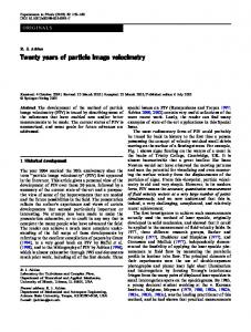
4 Results Two photographs of a section of the simulated downburst flow are presented in Fig. 4. Both the surrounding and the ambient fluids are seeded. In Fig. 4a, the indices of refraction of the two fluids are not matched. Note that the heavier downburst fluid is differentiated clearly from the ambient fluid. Although the seed particles in the ambient fluid are in focus, the seed particles in the downburst fluid are either blurred or completely faded. In Fig. 4b, the refractive indices of the two fluids are matched using the technique described in the previous section. It is difficult to detect any boundary or mixing zone between the two types of fluid, and the entire field of view is in focus. The index-matched photograph represents a section from a typical negative used for PIV analysis. Figure 5 shows a sequence of velocity fields in an evolving downburst obtained using PIV. Figure 6 shows the corresponding vorticity plots. The length scale R0 is o.o39 m, the time scale To is o.36 s, and the velocity scale V0 is O.ll m/s. Approximate times from release T/To are: 1.65, 3.86, 4.96, and 6.06. The initial height measured from the bottom of the cylinder is 2.86Ro. The flow Reynolds number, as defined previously, is 36oo. The spacing between vectors is approximately o.o6Ro. The vector plots shown represent raw data. Hence, no smoothing or interpolation of the data was performed. Figures 5a and 6a show the simulated downburst shortly after release. The maximum vertical velocity within the downburst fluid is 1.4V0 and occurs near the leading edge of the descending fluid. The uniform velocity vectors across the upper boundary and also within the downburst show minimal disturbance due to the breakage of the retaining membrane. The vorticity plot in Fig. 6 (a) shows development ofvorticity near the leading edge of the descending fluid. In Figs. 5b and 6b the downburst impinges on the horizontal plate. By this time, the maximum vertical velocity has increased to 2.1V0. This maximum vertical velocity occurs along the central axis of the downburst at a height of about 1.3R0 above the plate. Figure 5b shows entrainment of ambient fluid into the descending column and also shear instabilities at the interface between the two fluids. Figure 6b shows presence of vorticity at the interface between the lighter and heavier fluids. This vorticity is most intense near the leading edge of the descending parcel. In Figs. 5c and 6c the leading vortex ring has impinged on the plate and is expanding outward at a velocity of approximately o.sV0. The largest horizontal velocities occur near the ground and slightly aft of the core of the vortex ring. The maximum surface velocity is about 2.3V0 which is approximately five times greater than the propagation velocity of the ring. This is consistent with the computational model of Lundgren et al. (1992) where surface friction was included. The largest vertical velocity is still about 2.1Vobut occurs at a height of o.7Ro above the plate. Secondary vortices with opposite circulation (countervorticity) have been generated by friction at the surface of the plate. These weaker vortices are swept forward and upward by the primary vortex and can be seen just downstream of the advancing front in Fig. 6c. In computational studies, it was shown by Proctor (1988) and Lundgren et al. (1992) that these secondary vortices have a significant effect in shaping the structure of the outflow.

Fig. 4. a PIV picture without index matching; b PIV picture with matched indices Figures 5d and 6d show the next flame of the sequence as the vortex ring continues to propagate radially outward. The vorticity has intensified compared with the previous figure. Coherent counter-rotating vortices persist and have become stronger. The maximum vertical velocity has subsided to 1.1Vo within the descending column, and the downdraft shaft has become disorganized. Strong horizontal velocities persist beneath the vortex ring with a maximum of 1.5V0 again in the region closest to the ground and slightly upstream of the primary vortex ring. Both Figs. 6c and 6d show that there is little loss of vorticity to the wake. This was also observed in the Lundgren et al. (199z) flow visualization photographs. Lundgren et al. (1992) established the length and time scales for the microburst associated with the fatal crash of Delta Airlines Flight 191 (DL 191) near Dallas-Fort Worth airport in 1985. These scales were Ro = 0.7 km and TO= 23 s yielding a velocity scale of 30.4 m/s for this microburst. Using this scaling, we can determine how the simulated microburst relates to the DL 191 microburst. The release height of 2.86R0 corresponds to a height of 2000 m in the atmosphere. This is a reasonable height since the cloud base was at 185o m at the time this microburst occurred (Fujita 1986). The maximum surface velocity of 2.3 Vo scales to a 70 m/s wind velocity near the ground. These large velocities are present up to heights equivalent to 200 m in the atmospheric microburst and could be expected to pose significant problems for aircraft encountering them.

-

...~Vo . . . . . . . . . . . . . . . .

,~I

. . . . . . . . . . . . . . . .

~11

i,/

~,

IIII

...............

,~j~,~l

. . . . . . . . . . . . . . .

,/111~

. . . . . . . . . . . . . . . .

2

4 ~ Xl

ItlllJll,,l,+,

/

ttJ~

~l/~l~tz~,':::':':~;"'::::::::

I]ll l

tlz

~.-V o

. . . . . . . . . . . . . . . . . . . . . I . . . . . . . . . . . . . . . . . . . . .

I I I I I l l l l l l l l

. . . . . . . . . . . . . . . . . . . .

~

. . . . . . . . . . . . . . . . . . . .

i!ii!!iiiii!iiiii!!iiii:iiiiiiiiiiiiiiiiiiiiiiiii!!!!!iiii!iii!i!: J .'::::::;::::::::;;;~"~" ::::::::::::::::::::::

~;;;;~::;:::::::::: ~'~l~t/;:::;:;::iiiiiiiii

~

===================== ................ ....... ..........

:. .: .: .:.:.:.:.:.:.:.:. :. :. :. .: .: .: .:.: :

iii~i~i~i~iii!!!tt! : : : : : : : : : : : : .: :. :. :.: .: :. :. :.: .: :. :. : :

" ~/ /

]

::::::::::::::::::::

v

N

.~/z~. .......................

~ ,H~,

X

'

::~

..................

( " f " i

"i"

1"

"l'"f"

"f'Ji

"'1'

Ji""

7"'h'"

"F'+[

'i

"'i'"i"h'"

q,'h

v,

........

::::"

:

;IttB ..................... ; ' ~'::::::::::::::i: z~t { , . . .. . .. .: . .. .. .. . . . . . .

lz , ,zzz ~

. . .. .. .. .. .. .. .. .. .. .. .. .. .. .. .. ..

0

......................

z///-'-:::

~fi:'::": !ii'. ; ~;; : :: : : : :: ~, ~ ; ; ; ; . . . . . . . . . . . . . . . . . . . . .

1

a

.

~;;: ......................

~

~I ~

,x

:::::::::::::::::~, ":::::::::ii:::::~ iiiiiii!ii::i;ii

. . . . . . . . . . . . . . . . . . . .

/~]

........................

,x

.- . . . . . . . . . . . . . . .

::::.::::i::::::::::

}

::'

"r"r-t-'t'-

:,,,, ....

~'~F..r';I,

439

t----~ "r " ' , " ~ " ' ~ " ~ : ~ "

b 3

--,-.Vo

. . . . . . . . . . . . . . . . .

" ' z ~ l l l * * ' * * * ~ l * t ¢ l t ' ' l + + "

...................

,,,,,,,,,,,,,,,***,,,

.....................

2

~,,J,

:::::::::::::::~)}~

I[l 1111

ii t i l l

..................

+

]

~

............

" i i' i i. i .i i. i .; i. i .i i.i .

I III

~I~;:::-::::--::::.--:;: ........

. . . . . . .. . .. .x.. . ..I ' .' l .l.l l.i l..l ~. .. . .. .+ . ++++++++}+ill+ill++ . . . . . . . . . . . . + . ... .+ ..t ..... ......... ..... ..... . . .I /

" +f+~I ' X.

+ t + H l t t l t

, , ,

. . . . . . . . . . . . . . . . . . . . . . . . . . . .

,~+.~+,,l++~e+e+++l++++++*

. . . . . . . . . . . . . . . . . . . . . . . . . . . . . . .

.......

. . . . . . .

.........

I

l"l l 'l l l"l '

. . .. . .. ... ... ... .. . .. . .. . .. . .. . .. . .. . .. . .. . .. ... ... . . . . . . . . . . . . . . . . .

. . .. . .. ... .. . .. ... .. . .. . .. ... .. . . . . . . .

. . . . . . . . . . . . . . . .

r ............... ~* ] ~

]

, .................................................... +

~

.......... . . . . . . . . .

fl

.~].

"''

iii

. . . . . . . . . . . . . . . . . . . . . . . . . . . . . .

,, ..................................

/+I x+ ~ " ~ + ~ Ill

_. . . z. ." ' : , . . . .. . . . . [. ..... . . . . . . . ~, I~t , . . . . . /. . . . . . . . . . . . . ., t. ,. ,. x - - " ~ , l' /"I I I '

II

IIIII

..................

- . . . . . . . . . . . .

~ - ~ . . . ..... ..... ..... .. ... . +~

l' l l~l ' l 'l "

i~i14%~

. . . . . . . . . . . . . . . . . . . . t~,s++Xilll I Itlllllllll . + x l ~ ~l t l, l l l l l ~l tl ~l , l l l l l t, ,l+ , . . . . . . .. .. . . . .. .. . . . ..

::::::::::::::::::::::::::::

, J ~- U ~ | | H

. . . . . . . . . . . . . . . . . . . . . . . . . . . . . .

,llllltllll IlIIIJIIJIIITII IIJIIIIIIIIIIIIIIII+IJIIIILtl

. . . . . . . . . .

,,...,,,~'"':=:::::::"",, ," . . . . . . . . .f f~ . ..... . . . . . .......... . . . . . . . . .,.,. ... ... ... . . . . . . . . . . . . . . . . . . .x.',~; ..............

! i i ; ;#:#:t ,;~;l 1: 1: 1; 1; 1;1:+:,:l l:l : ; ; : : :

. . . . . . . . . . . . . . . . . . . . . . .

. . '.` .' '. ~ #. I./~I I Im ] z .~ . .- .- .- .- -. -. `. -. -. -. -. -.-.. + .... ~ff~ .....................

....',,

. . . . . . . . . . . . . . .

:::::::::::::::::::::::::::::: ::::::::::::::::::::::::::

'

. . . . . .

Illtll"

. ... .. ... .. ... .. .. . .. .. . .. .. . .. .. . .. .. . .. .. . .. .. . .. .. . .. .. . .. .. . .. .. . .. .. ... ..

iiI

.................... . . . . . . . . . . . . . . . . . . . . . . . . . . . . .. . .. .. . . . . . . . . ,.i t + .

;;;;:::ii:::

~+...,. . .... . . . . . .~. .,...,... ,. .H. .z. ~ - , z /

~lsJ"

;:::::;;::::::;;

I I . . . . . . . . . . . . . . . . . . . . . . . . . . . . . . I . . . . . . . . . . . . . . . . . . . . . . . . .

]] Ill

z

~

. . . .

. . . . . . . . . . .

.....................................

lllll++r flits"

llllll

"~l~lllll!t~tlI~lllll

. . . . . . . . . . . . . . .

1

j

;X++llllllllllllllJl x,~llllllllll

. . . . . . . . . . . . . . . .

,..~

l¢lllllllllll

= . . . . . . . . . . . . . . .

. . . . . . . . . . . . . . . . . . . . . . .

~,,,~,~m*~*J

. . . . . . . . . . . . . . . . . . . . . . ,,i[~[pllll

. . . . . . . . . . . . . . . . . . . . . . . . . . . . . . . . . . . . . . . . . . . . .

.....

"-'Vo

..........................................

llllllllllllllllllllll~l#*-

. . . . . . . . . . . . . . . . . .

-

~+, IIII

+I ~l +l ~l +l +l +l +l ' t+ l

: ....

l •. . . . .. . . .. . . .. . . .. . . .. . ... . ... . ..

.

.

.

.

.

~l l l l~l +l l~l , , . . . . . .• . i i , . - . . . . . . . . . . . . , , ~ t f , ~ .,.~. . , . . ,,. . . . . . .,.. . . .......... . . . . . .... . . . . . . . . . ,II~ .. .. .. .. . .;.".I. . . .. .. .. .. ........... .. .. .. .. .... . . . . . . . t. ~ t Y " ;

I~ ... ... . . . +. . ' . ' . ' . / / [~ [] ]/ "l l l l' l' 'l ' l ' l' l l . l .l .i .l *. .' r. . .. .. .. .. . . . . . . ... . .. . . . .

~ -:--~SX ..... ~ '.". . . . . . V . . ~.".'.' . . .. ..... . . .". ./ .Z. T ._./. ~. .H . .~. .s. ~. .t.l.t. . .~. . . . xx~' . . . . . . ..... . . . ./. . . .

: ....

I :J ~

'

1

""

.

.

.

.

.

.

X~

,4

.

.... f'::::

" ~ / / /+z

. . . . . . .

~ x ~ . . ~ , , ~ A / / ~ .. ~. :. . .

:. .: .' :. .

:

0 -1

O

1

2

r (Ro)

0

Fig. 5 a - d . Velocity fields o f a s i m u l a t e d m i c r o b n r s t o b t a i n e d u s i n g PIV. Ap/p=o.o3,

Ho/Ro=2.86, Re=36oo.

-1

0

d

1

2

r (Ro)

a 1.65; b 3.86; c 4.96; d 6.o6

A p p r o x i m a t e t i m e s T/To f r o m release.

The plots in Figs. 5b-d show that the peak horizontal velocities are reached at a radial position of approximately 1R0 at about 1 time unit after touchdown and that the velocities decay thereafter. Therefore, it is not surprising that the maximum velocity detected by the National Weather Service anemometer located approximately 5000 m (7Ro) to the south of the DL 191 microburst center was only 23 m/s. The experimental results thus imply that the strong gradients present cause difficulties in measuring the true strength of microbursts using ground-based anemometers. 5 Summary

Similar to other optical diagnostic techniques, PIV suffers from undesirable effects associated with variations in the index of refraction within the flow. In this experiment, this problem is overcome by matching the refractive indices of the lighter and the heavier fluids. Glycerol and potassium dihydrogen phosphate are used to obtain two solutions with a significant density difference but matched refractive indices. This combination is

easy to handle and works well for PIV measurements which require very precise matching. We expect it to work well also with other diagnostic techniques such as LDV. If larger quantities of the heavy solution are required, less expensive salts could be substituted for potassium phosphate. The effectiveness of the method is demonstrated by applying particle image velocimetry to a model microburst in order to obtain instantaneous maps of the velocity field with a high degree of accuracy and resolution. A microburst is modeled by releasing a small volume of heavy fluid into a large tank filled with a lighter fluid. The descending fluid impinges on a horizontal plate which represents the ground. The flow contains a pattern of coherent primary and secondary vortices. Although the flow is quite complex, it is dominated by a large primary vortex ring which forms near the leading edge of the downdraft. The vorticity intensifies after the vortex impinges on the bottom surface and expands radially outward. The PIV data are related to the behavior of full-scale atmospheric microbursts. The data scaled to the DL 191 show wind velocities as high as 7o m/s beneath the primary vortex

//

3

2

i',,

vortieity

/I

o

15 12.5 10

7.5 S

"'2", I ' II1¢ i1 ~

2.5 -2.$

',',

-5

1

-7.5 -10

44o

,C,

t',;,,

;/

;

o',

",L,

-12.5 -15

0

I

I

I

,

I

,

,

I

,

,

,

,

I

,

r

,

,

I

r

b

0 /

(?

~>

$

0

V

N tt ii

"-i ,-.

i s ¢t

:'~ ~-.I