Particle Swarm Optimization: Algorithm and its Codes in MATLAB Mahamad Nabab Alama a Department
of Electrical Engineering, Indian Institute of Technology, Roorkee-247667, India
Abstract In this work, an algorithm for classical particle swarm optimization (PSO) has been discussed. Also, its codes in MATLAB environment have been included. The effectiveness of the algorithm has been analyzed with the help of an example of three variable optimization problem. Also, the convergence characteristic of the algorithm has been discussed. Keywords: Algorithm, Codes, MATLAB, Particle swarm optimization, Program.
1. Introdunction Particle swarm optimization is one of the most popular nature-inspired metaheuristic optimization algorithm developed by James Kennedy and Russell Eberhart in 1995 [1, 2]. Since its development, namy variates have also been develop for solving practical issues of related to optimization [3, 4, 5, 6, 7, 8, 9, 10]. Recently, PSO has emerged as a promising algorithm in solving various optimization problems in the field of science and engineering [11, 12, 13, 14, 15, 16, 17, 18, 19, 20, 21, 22, 23, 24, 25].
2. Particle Swarm Optimization: Algorithm [25] Particle swarm optimization (PSO) is inspired by social and cooperative behavior displayed by various species to fill their needs in the search space. The algorithm is guided by personal experience (Pbest), overall experience (Gbest) and the present movement of the particles to decide their next positions in the search space. Further, the experiences are accelerated by two factors c1 and c2 , and two random numbers generated between [0, 1] whereas the present movement is multiplied by an inertia factor w varying between [wmin , wmax ]. The initial population (swarm) of size N and dimension D is denoted as X = [X1 ,X2 ,...,XN ]T , where 0 T 0 denotes the transpose operator. Each individual (particle) Xi (i = 1, 2, ..., N ) is given as Xi =[Xi,1 , Xi,2 , ..., Xi,D ]. Also, the initial velocity of the population is denoted as V = [V1 ,V2 ,...,VN ]T . Thus, the velocity of each particle Xi (i = 1, 2, ..., N ) is given as Vi =[Vi,1 , Vi,2 , ..., Vi,D ]. The index i varies from 1 to N whereas the index j varies from 1 to D. The detailed algorithms of various methods are described below for completeness. ∗ Mahamad
Nabab Alam Email address:
[email protected] (Mahamad Nabab Alam)
Preprint submitted to Open Access Article
March 8, 2016
k+1 k k k Vi,j = w × Vi,j + c1 × r1 × (P bestki,j − Xi,j ) + c2 × r2 × (Gbestkj − Xi,j )
(1)
k+1 k+1 k Xi,j = Xi,j + Vi,j
(2)
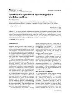
In eqn. (1) Pbestki,j represents personal best j th component of ith individual, whereas Gbestkj represents j th component of the best individual of population upto iteration k. Figure (1) shows the search mechanism of PSO in multidimensional search space.
Xik+1
Vik
Vik+1 Gbestik Vi
Xik
Gbest
Pbestik ViPbest
Figure 1: PSO search mechanism in multidimentional search space.
The different steps of PSO are as follows [25]: 1. Set parameter wmin , wmax , c1 and c2 of PSO 2. Initialize population of particles having positions X and velocities V 3. Set iteration k = 1 4. Calculate fitness of particles F ki = f (Xki ), ∀i and find the index of the best particle b 5. Select Pbestki = Xki , ∀i and Gbestk = Xkb 6. w = wmax − k × (wmax − wmin )/Maxite 7. Update velocity and position of particles k k k k k V k+1 i,j = w × V i,j + c1 × rand() × (P besti,j − X i,j ) + c2 × rand() × (Gbestj − Xi,j ); ∀j and ∀i k+1 k+1 k Xi,j = Xi,j + Vi,j ; ∀j and ∀i
8. Evaluate fitness Fik+1 = f (Xk+1 ), ∀i and find the index of the best particle b1 i 9. Update Pbest of population ∀i If Fik+1 < Fik then Pbestk+1 = Xk+1 else Pbestk+1 = Pbestki i i i
2
10. Update Gbest of population k+1 If Fb1 < Fbk then Gbestk+1 = Pbestk+1 and set b = b1 else Gbestk+1 = Gbestk b1
11. If k < Maxite then k = k + 1 and goto step 6 else goto step 12 12. Print optimum solution as Gbestk The most commonly used parameters of PSO algorithm are considered as follows: • Inertial weight: 0.9 to 0.4 • Acceleration factors (c1 and c2 ): 2 to 2.05 • Population size: 10 to 100 • Maximum iteration (Maxite): 500 to 10000 • Initial velocity: 10 % of position A detailed flowchart of PSO considering the above steps is shown in Figure (2). Set parameters of PSO
Initialize population of particles with position and velocity
Evaluate initial fitness of each particle and select Pbest and Gbest
Set iteration count k = 1
Update velocity and position of each particle
Evaluate fitness of each particle and update Pbest and Gbest
k = k+1
Yes
If k