tracing in the Cartesian space Strid et al., 1989]. A more detailed description of this method was recently given in Shirayama, 1993]. In most papers on particle ...
Particle Tracing Algorithms for 3D Curvilinear Grids I. Ari Sadarjoen
Theo van Walsum Frits H. Post
Andrea J.S. Hin
Delft University of Technology, Faculty of Technical Mathematics and Informatics, Julianalaan 132, 2628 BL Delft, The Netherlands This paper presents a comparison of several particle tracing algorithms on curvilinear grids. The fundamentals of particle tracing algorithms are described and used to split tracing algorithms into basic components. Based on this decomposition, two di�erent strategies for particle tracing are described in greater detail: tracing in computational space and tracing in physical space. Accuracy and speed tests are performed for both types of algorithms. From these tests it is concluded that particle tracing algorithms in physical space generally perform better than algorithms in computational space.
Keywords: scienti c visualization, vector eld visualization, particle tracing, interpolation, grid transformation
1 Introduction Computational Fluid Dynamics (CFD) is concerned with modelling uid ows. Increasingly sophisticated software is being developed to simulate interesting ow phenomena. Scientists can gain insight in the resulting data by visualization. One method of visualizing a velocity eld is particle tracing, which involves releasing particles into a ow and calculating their positions at speci c times. In general, CFD simulations provide a velocity eld de ned on a discrete grid. The simplest grids are block-shaped with cubical cells. Particle tracing algorithms for such Cartesian grids are investigated in [Yeung & Pope, 1988; Kontomaris & Hanratty, 1992]. In CFD practice, the grids are often boundary- tted and therefore curvilinear, with the purpose of solving ows in complex geometries. Particle tracing algorithms for CFD grids were presented in [Buning, 1989; Buning, 1988]. Some algorithms transform a curvilinear grid to a Cartesian grid and perform particle tracing in the Cartesian space [Strid et al., 1989]. A more detailed description of this method was recently given in [Shirayama, 1993]. In most papers on particle tracing, the scope is limited to a single method. If alternatives are given at all, they are not closely examined. Often, not all details of the particle tracing process are given, suggesting that some operations are straightforward. In commercial visualization packages, background information concerning the applied algorithms is seldom given. The present paper addresses the above issues. Detailed descriptions are given of the particle tracing process, which is split into distinct components. The strengths and weaknesses of di�erent implementations of these components are studied and visualized. The main aspects considered are accuracy and performance. After covering the fundamentals of particle tracing in section 2, the details of two di�erent classes of particle tracing algorithms will be described in section 3 and 4. Considerations for the implementation of several algorithms, as well as an overview of test cases are given in section 5. The test results and a discussion are presented in section 6. Finally, section 7 derives some 1
conclusions.
2 Fundamentals of particle tracing Although many terms are in use for grid types, we will reserve the term Cartesian grids for grids with straight grid lines and unit cubes as cells, and curvilinear grids for grids with curved (or more precisely: piecewise straight) grid lines and a regular topology. We will start by explaining the principles of particle tracing in Cartesian grids.
2.1 Cartesian grids
The computation of a particle path is based on a numerical integration of the ordinary di�erential equation dx = v(x) (1) dt where t denotes time, x the position of the particle and v(x) the velocity eld. The starting position x0 of the particle provides the initial condition:
x(t0 ) = x0 The solution is a sequence of particle positions (x(t0 ); x(t1); : : :).
(2)
A particle tracing algorithm must perform the following steps. First, a search is performed for the cell which contains the initial position of the particle. To determine the velocity at this position, the velocities at the cell corners are interpolated. Then, an integration step calculates the next position of the particle. Again, a search is performed, this time for the cell containing the new position. The process of interpolation, integration and point location is repeated until the particle leaves the grid. This process can be translated into pseudo-code representing the general structure of a particle tracing algorithm: find cell containing initial position particle in grid determine velocity at current position calculate new position find cell containing new position
while
endwhile
(point
location)
(interpolation) (integration) (point location)
Note that the above pseudo-code is merely intended to show the main algorithm components; in real implementations many re nements and optimizations could be made.
Point location
Determining which cell contains a speci ed point is called point location. The coordinates of a point can be divided into their integer and fractional parts: x = (x; y; z ) = [i; j; k] + (�; ; ), where i; j; k are integers and �; ; 2 [0; 1]. In paper, we will refer to [i; j; k] as the indices and (�; ; ) as the o�sets. Point location in a Cartesian grid is as simple as truncating the coordinates to their integer parts. Here, determining the o�sets is also considered to be part of the point location operation, but sometimes we will strictly distinguish between point location and o�set determination.
Interpolation
To obtain a value of the velocity eld at other points than the grid nodes, it is necessary to determine an interpolated value from the nodes surrounding the point. The standard way to do this in cubical cells is trilinear interpolation. This requires the cell indices and the o�sets 2
obtained through point location. Let I; J; K 2 f0; 1g and let the basis functions be de ned as 0 (�) = 1 ? � and 1 (�) = �. Then, for a point x in a cell [i,j,k] with o�sets (�; ; ), the function T determines the interpolated value from the corner velocities vi;j;k : : : vi+1;j +1;k+1.
v = T (v; �; ; ) =
1 X
I;J;K =0
vi+I;j+J;k+K � I (�) J ( ) K ( )
(3)
Integration
Many integration methods are known in the literature, ranging from the simple rst-order Euler scheme to the fourth-order Runge-Kutta scheme or even higher-order methods, applied with xed or variable time steps. A well-known second-order method is Heun's scheme, also known as a second-order Runge-Kutta scheme. Starting from position xn at time t = tn , the position xn+1 at time t = tn+1 is calculated in two steps: x�n+1 = xn + �t � v(xn) (4) � (5) xn+1 = xn + �t � 21 v(xn) + v(x�n+1 )
2.2 Curvilinear grids
In practice, the grids used in many CFD applications are not Cartesian. To handle complex geometries, curvilinear, boundary- tted grids are used. These grids are also referred to as structured grids, because they have a regular topological structure, as opposed to unstructured grids as used in Finite Element Methods. While this allows for a large variety of geometries, numerical procedures are more di�cult in curved grids. This is the reason why in CFD ow solvers, the curvilinear grid in the physical domain is often internally transformed to a Cartesian grid in a new domain. The physical domain will be called P-space (P ) and the new domain will be called computational space or C-space (C ). Many calculations are performed more e�ciently in the simple Cartesian grid in C-space. In particle tracing in a curvilinear grid similar problems arise. Especially point location and interpolation become more complex. This suggests the use of a similar procedure in determining particle paths for visualization purposes as for ow solving. A transformation is de ned from physical space to computational space such that the curvilinear grid becomes a Cartesian grid (see gure 1). ζ z η ξ
(i, j, k)
x
(i, j, k)
y
computational space (ξ,η,ζ)
physical space (x,y,z)
Figure 1: Transformation between P and C In a Cartesian grid, point location and interpolation can be carried out as described in the previous subsection. We must transform the positions of the complete path back to the physical domain to be able to visualize it, but the use of the convenient computational domain may increase the e�ciency of the algorithm. The details will be discussed in section 3. 3
An alternative is to calculate the particle path directly in P-space (P ). This would involve more complex point location and interpolation, but would avoid grid transformation. This alternative will be covered in section 4.
2.3 Restrictions
We will restrict our attention to stepwise integration methods. Also, we will only use the secondorder Runge-Kutta method with xed time steps. For reasons of simplicity, we consider the ow eld to be time-independent. A paper that discusses visualization of time-dependent ow elds is [Lane, 1993].
3 C-space algorithms Particle tracing in computational space proceeds in almost the same way as described in section 2.1, except that the physical velocities v must be transformed to u in C and instead of equation (1), the following di�erential equation is solved: d� = u(�) (6) dt where � denotes a position in C . The solution is now a sequence of positions (�(t0 ); �(t1 ); : : :) in computational coordinates. As a consequence, the particle path calculated in C must be transformed to physical space for visualization purposes. The general form of the algorithm then becomes: find cell containing initial position particle in grid transform corner velocities from P to C determine C-velocity at current position calculate new position in C-space transform C-position to P find cell containing new C-position
while
endwhile
(point
location)
transform velocities)
( (interpolation) (integration) ( (point location)
transform position)
The point location and interpolation parts in this algorithm are straightforward, because the computational grid is Cartesian. However, from the pseudo-code it can be seen that two transformation operations are introduced. First, the physical velocities must be transformed to C-space. Second, the calculated particle positions must be transformed back to P-space. The former operation is not necessary if it is possible to use the velocities in computational space that are used during the ow solving process. However, we also assume that the results from the ow solver are physical velocities. It should be emphasized, that in the above algorithm the velocity eld is not transformed and stored in its entirety, but only the velocities in the current cell are transformed on-the- y. In other words, they are local transformations, since in most of the cases no single, global grid transformation from P to C exists.
3.1 Transformation of positions from C to P
The transformation of a position from C to P is relatively straightforward. What is necessary, is a transformation which maps the corner nodes of a cubic cell in computational space to the corner nodes of a cell in physical space. The edges between nodes are assumed to be straight in either space. This leads to a transformation which is equivalent to a trilinear interpolation between the cell corner P-space positions, as in equation (3). The function T transforms a C-space position � = (�; �; � ) consisting of integer parts [i; j; k] and fractional parts (�; ; ) to a P-space position x as x = T (x; �; ; ) (7) 4
3.2 Transformation of velocities from P to C .
A velocity u in C is transformed to v in P according to: v = J�u and similarly, a velocity v in P can be transformed to u in C with u = J?1 � v The matrix J is called the Jacobian and contains the partial derivatives: 0x x x 1 � � � J = @ y� y� y� A z� z� z�
(8) (9) (10)
where x� is short for @x @� etc. The matrix J can be thought of as consisting of the columns (j1 j j2 j j3 ). These are in fact the partial derivatives @@�x ; @@�x ; @@�x . As we are dealing with (discrete) grids, the Jacobian must be calculated with nite di�erences. There are several methods for doing this. Another aspect is the number of Jacobians used for each cell.
Jacobian approximations
To approximate a Jacobian in a grid point, several types of di�erencing are available. Given the coordinates of the grid nodes xi;j;k where [i; j; k] lie within the grid boundaries, there are at least three possibilities: � forward di�erences: j1 = ��x� = xi+1;j;k ? xi;j;k
� backward di�erences: j1 = ��x� = xi;j;k ? xi?1;j;k � central di�erences : j1 = ��x� = (xi+1;j;k ? xi?1;j;k)=2 Calculating the derivatives j2 = ��x� and j3 = ��x� proceeds in a similar way.
In a 2D cell, these di�erences can be combined to the cases in gure 2. In an arbitrary grid node ( gure 2a) either forward di�erences ( gure 2b), backward di�erences ( gure 2c) or central di�erences ( gure 2d) can be calculated. Alternatively, mixed di�erences, such as forward for j1 and backward for j2 ( gure 2e), or vice versa ( gure 2f) can be used.
Number of Jacobians
The other aspect is the number of Jacobians calculated in a cell. Basically, there are three options: � one for each cell (see gure 3a) � one for each node (see gure 3b) � one for each node for each adjacent cell (see gure 3c) The simplest and fastest method is to calculate only one Jacobian per cell [Strid et al., 1989]. By computing forward, backward or central di�erences in one node, for example in the lower left node, it is assumed that this Jacobian reasonably represents the deformation throughout the entire cell (see gure 3a). Another approach is to calculate separate Jacobians in each grid node [Shirayama, 1993]. Now, four di�erent Jacobians have to be calculated in a 2D cell (see gure 3b), or eight in a 3D cell. Using mixed types of di�erences leads to one Jacobian per node per adjacent cell. The Jacobian for a node is calculated according to which cell the particle is in. We shall call this forward/backward di�erences (see gure 3c). 5
j_1 j_1 j
j_2
j_2
i
a
b
c j_1
j_1 j_2
j_2
j_2
d
j_1
e
f
Figure 2: Several types of di�erences for Jacobian calculation
J_bdbd
J_cd J_cd
J_bdfd J_cd
J_fdbd
J_cd
a
J_cd
b
J_fdfd
Figure 3: Number of Jacobians in a 2D cell
6
c
This method of calculating Jacobians is mathematically correct when trilinear interpolation is used for point transformation. We give more details on this in the Appendix. The results have been con rmed by other researchers who have found similar results [Kenwright, 1994].
4 P-space algorithms The alternative to particle tracing in a simple Cartesian grid in C-space, is particle tracing in a complex curvilinear grid in P-space. This has a considerable impact on the complexity of the algorithm presented in section 2. In particular, point location and interpolation are not straightforward. There is no longer a simple relation between a physical position in space and the grid cell that contains it. Moreover, as the cells in a curvilinear grid are not cubes, it is also not as easy to perform trilinear interpolation, because the relative position (fractional o�sets) of a position in a cell is hard to determine. The next two subsections will discuss alternative point location and interpolation methods, respectively.
4.1 Point location methods
We can distinguish between global and incremental point location. In global point location, a given point in a grid must be found with no previous known cell. In a curvilinear grid this is not an easy task. As with all search algorithms it is possible to use a simple brute-force algorithm which searches all grid cells one-by-one. Naturally, this is expensive. Auxiliary data structures can be used to perform a smart search [Neeman, 1990; Williams, 1992]. Fortunately, particle tracing is a step-by-step process, in which, most of the time, global point location is only necessary to nd the cell containing the initial position of a particle. After this, there is always a current starting position and a current starting cell, from which the new position is to be found. This occurs at every integration step that starts from the current particle position in some known cell and calculates a new position. The following paragraphs will discuss only incremental point location.
Tetrahedrization
To use tetrahedrization, the curvilinear hexahedral cells are decomposed into tetrahedra. The reasons for this are: 1. Tetrahedra are convex, which facilitates testing if a speci ed point is inside. 2. Tetrahedra have planar faces, which facilitates intersection with a line. Incremental point location can now be performed by drawing a line from the previous known position to the next position [Garrity, 1990]. Intersections with the faces of the tetrahedron and containment tests in neighbouring cells are used to locate the new point. Tetrahedrization is only performed in the cells along the path of the line and the results do not have to be stored, nor does the tetrahedrization involve insertion of new grid points.
Stencil Walk and Newton-Raphson Let P be a point given in physical space that must be found in computational space. In the so-called stencil walk method [Buning, 1989], rst an initial point � in computational space is chosen. This point is transformed to physical space using the transformation x = T (x; �; ; ). The di�erence between the transformed point x and the target point P is calculated as �x = x ? P. This di�erence vector in physical space is transformed to computational space using �� = J?1 �x and added to the previous point, resulting in a new guess. If one of the elements of �� is outside the range [0; 1], the centre of the corresponding neighbouring cell is the new guess. The iterative process continues until the right cell has been found. Once the correct cell has been found, one can iterate until the value of �� is small enough. 7
We can also use the well-known Newton-Raphson iteration [Gerritsen, 1988; Mooiman, 1993] that nds the root to the equation F (� ) = 0 by the following relation: F (�) (11) �n+1 = � n ? 0 F (�) Here, F is de ned as F (�) = P ? T (� ), P is again the point in P-space to be found in C-space, and T is the function that transforms a point from C-space to P-space. Then, the derivative F 0 = ?T 0 is a Jacobian matrix, and the usually 1D division by F 0 turns into a matrix inversion in 3D. Experiments have shown that this method converges rapidly [Mooiman, 1993]. It can be shown that o�set calculation using a Newton-Raphson process is identical to o�set calculation using a stencil walk process, if the stencil walk algorithm uses interpolated forward/backward Jacobians for the transformation of �x. By substituting the above de nition of F into equation 11, taking into account that F 0 = J, the equivalence relation can be easily derived.
4.2 Interpolation methods
Trilinear interpolation
If the o�sets in the cell (�; ; ) are available, an interpolated velocity can be determined from the data values in the cell corners, as in equation (3). One way to determine (�; ; ) in a curvilinear grid is by using the Stencil Walk/Newton-Raphson iteration. The following two methods provide alternative ways of interpolation that do not require the o�sets.
Inverse Distance Weighting Let x0 ; : : :; x7 be the coordinates of the eight corner nodes of a hexahedral cell, and let v0 ; : : :; v7 be the velocities in those nodes. Then, the interpolated value v in point X is calculated as a
weighted average of the corner values [Wilhelms et al., 1990; Watson, 1992]: v = w 0 v 0 + w1 v 1 + � � � + w 7 v 7 (12) The weight of each data point is calculated as a function of the Euclidian distance between xi and X: di = kxi ? Xk (13) 12
(di ) wi = X 7
1 2 ( d j =0 j )
(14)
In a 2D cell consisting of four nodes, the same principle can be applied (see gure 4). Should X be close to a corner node, the distance di would be nearly zero and the value wi would be unpredictable. This is handled in the algorithm by testing whether the distance di is close to zero, in which case the weight of that corner is set to 1, and the weights of all other nodes are set to zero. The advantage of this method is that it does not require the fractional o�sets. The disadvantage is that the interpolated eld is discontinuous over cell boundaries.
Volume Weighting
In volume weighting, interpolation is performed within a tetrahedron, based on volume weights. Let X be a point in a tetrahedron consisting of nodes x0 ; x1 ; x2 and x3. Then, the tetrahedron can be subdivided into four tetrahedra, in all of which X is a corner node. The weight for each node of the main tetrahedron is the ratio of the volume of the subtetrahedron to the volume of the main tetrahedron [Buning, 1989]. X w1 = V023X w2 = V013X w3 = V012X w0 = VV123 (15) V0123 V0123 V0123 0123 8
x3 x2
d3
d2 X
d1
d0
x1
x0
Figure 4: Inverse Distance Weighting The volume of an arbitrary tetrahedron ABCD is calculated as ~ � (AC ~ � AD ~ )j (16) VABCD = 16 jAB This interpolation method can take advantage of the information created in decomposing cells into tetrahedra, if tetrahedrization is used as the point location method. The principle is demonstrated in 2D in gure 5, where the equivalent of tetrahedral volumes are triangular areas. The weight of node x0 is the ratio of the area A0 of the opposing subtriangle to the area of the main triangle. Volume weighting is continuous over the cell faces. x2
X
A0
x0 x1
Figure 5: Area weighting Note that in 3D only four nodes of the cell are used for the interpolation, since only one of the subtetrahedra forming the hexahedral cell is used, whereas in IDW or trilinear interpolation eight nodes are used.
5 Implementation and test ows Based on the descriptions in section 3, the algorithms listed in table 1 and 2 have been implemented. Table 1 lists the C-space algorithms. In all of these, point location and interpolation are straightforward as described in section 2. Only the transformation methods vary. In C-FD1, one Jacobian is calculated per cell using forward di�erences in one node. In C-FD8 and C-CD8, eight Jacobians are calculated per cell using forward and central di�erences, respectively. In C-FDBD, eight Jacobians are calculated per cell using mixed di�erences. Table 2 lists the P-space algorithms, each with a code of the form (P-xx-yy). Here, -xxstands for the point location method, and yy for the interpolation method used. P-T-IDW uses 9
Algorithm Transformation C-FD1 1 forward di�. per cell C-FD8 8 forward di�. per cell C-CD8 8 central di�. per cell C-FDBD forward/backward di�.
Algorithm Interpolation P-T-IDW Inv. Dist. Weighting P-T-VOL Volume Weighting P-SW-TRI Stencil Walk + trilin. Table 2: P-space algorithms
Table 1: C-space algorithms
the tetrahedrization (-T-) for point location and Inverse Distance Weighting for interpolation. P-T-VOL also uses tetrahedrization for point location, but uses volume weighting for interpolation. P-SW-TRI uses a Stencil Walk for point location, and trilinear interpolation with fractional o�sets obtained by the point location process. All implemented algorithms employ a second-order Runge-Kutta method as described in section 2. First-order methods (such as Euler) were found to be inadequate by several researchers [Buning, 1988; Shirayama, 1993]. Others use higher-order methods as well. But since the integration method was not our main point of interest, we did not implement these.
Test ows
Ideally, to test the algorithms, ows should be used for which it is possible to analytically calculate the path travelled by a particle. Given a particle starting position, it should be possible to calculate the particle position x(t) for any given time t. This allows for a comparison of the particle paths computed by the algorithms to the theoretical paths. Unfortunately, in 3D ows it is seldom possible to determine the analytical solution of a particle trajectory. This make it more di�cult to verify the accuracy of 3D particle paths. Therefore, we used only two-dimensional ows (although they were de ned on a 3D grid). Nevertheless, there is no reason to expect that the third dimension should behave di�erently from the other two. Altogether, in this study we used seven test ows: two 2D theoretical ows, two 2D CFD simulated ows and three 3D simulated ows [Sadarjoen, 1994]. In this paper we will present only two typical 2D examples, one theoretical and one simulated ow.
Uniform ow in straight pipe with curved grid
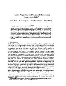
One kind of ow where the theoretical particle paths are known, is a uniform ow. This test ow is de ned on a 21 x 41 x 2 curvilinear grid, which originates from a practical CFD application (see gure 6). The grid represents a vertical pipe with an inlet located at the bottom and an outlet at the top.
Flow in L-shaped pipe
The second test ow uses an L-shaped pipe, in which the ow has been calculated using the ISNaS CFD-simulation package [Mynett et al., 1991]. The grid shown in gure 7 consists of 7 x 23 x 2 nodes and contains a sharp discontinuity. The inlet of the pipe is at the right (x = 2:5).
6 Test results
6.1 Transformation e�ect
The two test cases described above were used to test the e�ect of the transformation component in a C-space particle tracing algorithm. All C-space algorithms (C-FD1, C-FD8, C-CD8 and C-FDBD) were applied to these two problems. As a reference, a P-space algorithm (P-T-IDW) was used. 10
15
10
5
0 -0.05
-0.04
-0.03
-0.02
-0.01
0
0.01
0.02
0.03
0.04
0.05
Figure 6: Curved grid
5 4.5 4 3.5
y
3 2.5 2 1.5 1 0.5 0 0
0.5
1
1.5
2
2.5 x
3
Figure 7: L-pipe grid
11
3.5
4
4.5
5
Uniform ow in straight pipe with curved grid
As the ow eld is uniform, the particle paths should be straight vertical lines. All P-space algorithms produce this exact solution. Figure 8 shows the resulting particle paths calculated by the P-T-IDW algorithm. Since the velocity eld in P-space is constant, the P-space algorithms all give the same solution, so any other P-space algorithm could be used instead of P-T-IDW. The particle paths produced by C-FD1 are shown in gure 9; they are not straight. The other C-space algorithms produce similar inaccurate results.
Figure 8: Flow in straight pipe with curved grid. Straight particle paths P-T-IDW A closer comparison is possible when particle paths calculated by di�erent algorithms are combined in one gure. In gure 10 the particle paths produced by ve algorithms are combined and magni ed to highlight the di�erences. The straight solid line was produced by the P-space algorithm. The other solid line, closest to the other one, but with a few oscillations, was produced by the C-FDBD-algorithm. The other C-space algorithms show greater deviations, in particular C-FD1 and C-FD8. C-CD8 appears to be signi cantly more accurate, but C-FDBD still gives the best results. From these results the conclusion could be drawn that a simple transformation as described in [Strid et al., 1989] (C-FD1) or [Shirayama, 1993] (C-FD8) gives inadequate results.
Flow in L-shaped pipe
In the previous test, two C-space algorithms were found to be signi cantly better than the others: the C-CD8 algorithm which uses central di�erences and the C-FDBD algorithm, which uses forward/backward di�erences. These two algorithms were applied to the test ow in the L-shaped pipe. The integration timestep was set to 0.01, with up to 1000 time steps calculated. Figure 11 shows the result of the C-CD8 algorithm, gure 12 shows the result of the C-FDBD algorithm. Again, we observe that the results of C-FDBD are better than those of C-CD8, in spite of the fact that C-CD8 is a second-order method and C-FDBD a rst-order method. However, the di�erence between the two methods is that C-CD8 transforms the physical velocity eld into a continuous velocity eld in C-space, while C-FDBD transforms it into a discontinuous velocity eld. Since the 12
Figure 9: Flow in straight pipe with curved grid. Curved particle paths C-FD1
10 9 8
P-4-IDW C-FD1 C-FD8 C-FDBD
7
C-CD8
6 5 4 3 2 1 0 -0.0215
-0.021
-0.0205
-0.02
-0.0195
-0.019
-0.0185
Figure 10: particle path produced by di�erent algorithms
13
-0.018
Figure 11: Particle paths in L-shaped pipe; Algorithm C-CD8
Figure 12: Particle paths in L-shaped pipe; Algorithm C-FDBD
14
grid lines are not di�erentiable at the grid nodes, the transformed velocity eld in C-space must be discontinuous. We will return to this subject in the discussion (section 6.4).
6.2 Interpolation e�ect
To investigate the e�ect of the interpolation method on the accuracy of the particle paths, the P-space algorithms (P-T-IDW, P-T-VOL, P-SW-TRI) were examined. These algorithms di�er only in their interpolation components. Again, the ow in the L-pipe was used. The same particles as in the previous test were released and their paths traced. Figure 13 shows the results for the P-T-VOL algorithm. The results for the other P-space algorithms cannot be visually distinguished and are therefore not included.
Figure 13: Particle paths in L-shaped pipe; Algorithm P-T-VOL
6.3 Speed comparison
All algorithms were applied to the ow in the L-shaped pipe and total execution times were measured with timing routines. Table 3 lists the results in seconds. The platform used was a SiliconGraphics Iris 4D/310-VGX workstation. Algorithm P-T-IDW P-T-VOL P-SW-TRI Execution time 56.2 42.4 151.6 Algorithm C-FD1 C-FD8 C-CD8 C-FDBD Execution time 28.3 76.2 76.0 83.1 Table 3: Timing results
15
6.4 Discussion
Accuracy: interpolation
In general, the di�erences in accuracy between the P-space algorithms caused by various interpolation methods are marginal. Both the 2D and 3D test cases that we have used have shown this.
Accuracy: velocity eld transformation
The accuracy of C-space algorithms is largely determined by the transformation. C-FDBD is the most accurate algorithm. This can be explained from an analysis of the transformation based on a simple test case. Consider the uniform vector eld in the four curvilinear cells in gure 14. When transforming this vector eld to computational space, the vectors at the left and right borders (x = 0 and x = 3) are not a problem because the grid lines are di�erentiable there. The problem lies in the vectors in the middle of the grid, especially the vector in (2, 1). Now, assume that particles are released from (1; 0) and (2; 0). In P-space this would result in straight the particle paths in x = 1 and x = 2 (see gure 15). When these particle paths are transformed to C-space, we obtain the curved paths shown in gure 16. Note that here, not vectors are transformed, but positions on the paths, using the Newton-Raphson iteration described earlier. Consider the rightmost path, with a sharp transition at (1, 1). At the cell boundary, the direction of the path changes abruptly. Since the path contains grid node (1,1) and the velocity in a grid node is de ned entirely by the velocity in that node, this means that the velocity vector in (1, 1) must also change in the same way. In other words: the velocity eld must be discontinuous over cell boundaries. Consequently, the velocity in the corresponding point in P-space (2, 1) must map to di�erent vectors in C-space, depending on which cell the node belongs to. The transformation that has this property is FDBD, because di�erent Jacobians are used in a node, depending on the cell it belongs to. In other words: the continuous velocity eld in P-space must be transformed to a discontinuous eld in C-space. The reason for this, is that the grid lines are also discontinuous, since they are assumed to be straight lines connecting the grid nodes. This example also shows that the transformations which use either one Jacobian per cell or one Jacobian per node give less accurate results, even if they are second-order, such as the central di�erencing in the C-CD8 algorithm. It can also be veri ed analytically that the tangent vectors of the particle paths are correctly calculated, if all the vectors are transformed with FDBD.
Speed
C-FD1, which uses one Jacobian per cell, is the fastest algorithm. The other C-space algorithms are roughly six times as slow. This can be explained from the fact that eight Jacobians per cell are calculated rather than one. The P-space algorithms are in general faster than the C-space algorithms that use eight Jacobians, although the e�ciency of the C-space algorithms could probably be improved upon by applying some optimizations. Among the P-space algorithms, P-T-VOL is the fastest. Although the calculation of the weights is more complex in volume weighting than in inverse distance weighting, this disadvantage seems to be outweighed by the fact that only four weights in each cell need to be calculated, rather than eight.
7 Conclusions Particle tracing algorithms have been decomposed into their characteristic components. Various alternatives for these components have been implemented and compared. A distinction has been made between computational space (C-space) and physical space (P-space) algorithms. 16
2.5
2
1.5
1
0.5
0 -0.5
0
0.5
1
1.5
2
2.5
3
3.5
3
3.5
Figure 14: Uniform vector eld in four cells 2.5
2
1.5
1
0.5
0 -0.5
0
0.5
1
1.5
2
2.5
Figure 15: Straight particle paths in Pspace
2 1.8 1.6 1.4 1.2 1 0.8 0.6 0.4 0.2 0 0
0.5
1
1.5
2
Figure 16: Curved particle paths in C-space 17
The most important component in C-space algorithms is the transformation. Varying this component has a large impact on the accuracy of the results. Varying the interpolation component in P-space algorithms has much less e�ect on the results. The accuracy of C-space algorithms depends highly on the deformation of the grid. In Cartesian grids, C-space algorithms are identical to P-space algorithms. If the transformation is not calculated correctly, the accuracy of C-space algorithms decreases rapidly in deformed grids. Among the C-space algorithms, C-FDBD has turned out to be the best, both theoretically (see also the appendix) and experimentally. The reason for considering particle tracing in C-space was e�ciency. However, tests have shown that most C-space algorithms are computationally more expensive than P-space algorithms, at least when the data is provided in P-space. In general, P-space algorithms are more accurate and e�cient than C-space algorithms. The e�ect of varying the interpolation method is small compared to the transformation e�ect. Therefore, the use of C-space is less useful for particle tracing, but if a C-space algorithm must be used, the C-FDBD-algorithm is the best choice.
Acknowledgements
We wish to thank Arthur Mynett of Delft Hydraulics for his help and support and for his comments on earlier versions of this paper. We thank Jan Mooiman of Delft Hydraulics, for providing interesting data sets and for many useful discussions on uid dynamics. This work was supported by Delft Hydraulics.
18
References Buning, P. 1988. Sources of Error in the Graphical Analysis of CFD Results. Journal of Scienti c Computing, 3(2), 149{. Buning, P. 1989. Numerical Algorithms in CFD Post-Processing. In: Computer Graphics and Flow Visualization in Computational Fluid Dynamics. Lecture Series 1989-07. Von Karman Institute for Fluid Dynamics, Brussels, Belgium. Garrity, M. 1990. Raytracing Irregular Volume Data. Computer Graphics, 24(5), 35{40. Gerritsen, M. 1988. Geometrical modelling of 3D Aerodynamic Con gurations. M.Sc. thesis, Technische Universiteit Delft, Faculteit Lucht- en Ruimtevaart. Kenwright, D.N. 1994. Personal Communications. Kontomaris, K., & Hanratty, T.J. 1992. An Algorithm for Tracking Fluid Particles in a Spectral Simulation of Turbulent Channel Flow. Journal of Computational Physics, 103, 231{242. Lane, D.A. 1993. Visualization of Time-Dependent Flow Fields. Pages 32{38 of: Nielson, G.M., & Bergeron, D. (eds), Visualization '93. IEEE Computer Society Press. Mooiman, J. 1993. Personal Communications. Mynett, A.E., Wesseling, P., Segal, A., & Kassels, C.G.M. 1991. The ISNaS incompressible Navier-Stokes solver: invariant discretization. Applied Scienti c Research, 48, 175{191. Neeman, H. 1990. A Decomposition Algorithm for Visualizing Irregular Grids. Computer Graphics, 24(5), 49{62. Sadarjoen, A. 1994. Algoritmen voor particle tracing in 3D kromlijnige roosters. M.Sc. thesis, Delft University of Technology. In Dutch. Shirayama, S. 1993. Processing of Computed Vector Fields for Visualization. Journal of Computational Physics, 106, 30{41. Strid, T., Rizzi, A., & Oppelstrup, J. 1989. Development and Use of Some Flow Visualization Algorithms. In: Computer Graphics and Flow Visualization in Computational Fluid Dynamics. Lecture Series 1989-07. Von Karman Institute for Fluid Dynamics. Watson, D.F. 1992. Contouring: A Guide to the Analysis and Display of Spatial Data. Computer Methods in the Geosciences, vol. 10. Pergamon Press. Wilhelms, J., Challinger, J., Alper, N., & Ramamoorthy, S. 1990. Direct Volume Rendering of Curvilinear Volumes. Computer Graphics, 24(5), 41{47. Williams, P. 1992. Interactive Direct Volume Rendering of Curvilinear and Unstructured Data. Ph.D. thesis, University of Illinois. Yeung, P.K., & Pope, S.B. 1988. An algorithm for Tracking Fluid Particles in Numerical Simulations of Homogeneous Turbulence. Journal of Computational Physics, 79, 373{416.
19
Appendix Calculation of Jacobians
In this appendix, we take a closer look at the transformation of vectors between physical space P and computational space C . The following is based on the common assumption that points are transformed from C to P by trilinear interpolation. In a 2D cell with corner nodes A, B, C and D (see gure 17), this transformation is de ned as T (�; ) = I (A; B; C; D; �; ) = (1 ? �)(1 ? )A + �(1 ? )B + (1 ? �) C + � D (17) where � and are normalized coordinates in C . To transform vectors between P and C , the transformation Jacobian is used, a matrix with the partial derivatives of the transformation. These can be calculated either continuously or discretely. We will demonstrate that equivalence continuous Jacobians are equivalent the FDBD type of discrete Jacobians, when using trilinear interpolation in a cell.
Continuous Jacobians
In the continuous calculation of a Jacobian, the analytical derivative of the transformation is determined. This derivative is a 2x2 matrix with columns (j1 j j2 ) = ( @@�T j @@ T ). With the de nition of T as in equation (17), we can calculate the rst column as: @ I = ?(1 ? )A + (1 ? )B ? C + D = (1 ? )AB ~ + CD ~ j1 = @� With a similar calculation of j2 , we nd � � ~ + CD ~ j (1 ? �)AC ~ + �BD ~ Jcont(�; ) = (1 ? )AB (18)
Discrete Jacobians
In the discrete Jacobian calculation, di�erent Jacobians are calculated in di�erent corners, using nite di�erences as described in section 3.2. Next, the corner Jacobians are linearly interpolated, in order to correctly represent the cell deformation throughout the entire cell. We will describe how the three types of di�erencing a�ect the resulting Jacobians. Forward di�erences: In the case of the C-FD1-algorithm which uses 1 Jacobian per cell, we ~ j AC ~ ). Interpolating does not have any in uence in this case, have: JA = JB = JC = JD = (AB and the result is not equal to Jcont (equation 18). Central di�erences: In the approximation with central di�erences, the Jacobians in each node consist of columns with the averages of the edges connected to that node (see g. 17). In this case, the Jacobians in the respective corners are given by: ~ + AB ~ ) j 1 (QA ~ + AC ~ )) JA = ( 21 (PA (19) 2 ~ + BS ~ ) j 1 (RB ~ + BD ~ )) JB = ( 21 (AB 2 ~ + CD ~ ) j 1 (AC ~ + CU ~ )) JC = ( 21 (TC 2 ~ + DW ~ ) j 1 (BD ~ + DV ~ )) JD = ( 12 (CD 2 After interpolation, the rst column of the resulting Jacobian is: ~ + AB ~ ) + 1 �(1 ? )(AB ~ + BS ~) j1 = 21 (1 ? �)(1 ? )(PA 2 ~ + CD ~ ) + 1 � (CD ~ + DW ~ ) + 21 (1 ? �) (TC 2 � � � � ~ + (1 ? �)PA ~ + �BS ~ + 1 CD ~ + (1 ? �)TC ~ + �DW ~ (20) = 21 (1 ? ) AB 2 20
V
V
U
U D C
T
D
W
J_D
P
J_A
A
Q
C
T
J_C
S
J_B
J_D
J_C
P
J_A
Q
R
Figure 17: Jacobians with central di�erences
S
J_B
A
B
W
B
R
Figure 18: Jacobians with FDBD di�erences
This is di�erent from the rst column of Jcont (equation 18), so again the discrete Jacobian is not equal to the continuous one. Forward/Backward di�erences: in this case the neighbouring cells are not used. However, the approximating Jacobians are better, because within the appropriate cell they form a better representation of the cell deformation (see gure 18). Now, the Jacobians are given by: ~ j AC ~) JA = (AB (21) ~ ~ JB = (AB j BD) ~ j AC ~ ) JC = (CD ~ j BD ~ ) JD = (CD When these are interpolated, the resulting Jacobian is identical to Jcont:
Jdisc (�; ) = I (JA ; JB ; JC ; JD ; �; ) = (1 � ? �)(1 ~? )JA ~+ �(1 ? )JB~ + (1 ?~�)� JC + � JD = (1 ? )AB + CD j (1 ? �)AC + �BD
(22)
Hence, in contrast to forward or central di�erencing, FDBD-di�erencing gives a correct approximation of the transformation Jacobian within the cell; provided that trilinear interpolation is used for that transformation.
21