Proceedings of the 2001 Particle Accelerator Conference, Chicago
PARTICLE TRACKING ON UNSTRUCTURED GRIDS∗ E. M. Nelson† , LANL, Los Alamos, NM K. R. Eppley, J. J. Petillo, SAIC, Boston, MA B. Levush, NRL, Washington, D.C.
We report on recent developments and tests of a novel particle tracking algorithm. This algorithm tracks particles element by element through the unstructured grid, stopping and then restarting at each element boundary crossing. Within each element the particles are tracked in the element’s local coordinate system. Excellent accuracy is achieved with high order Runge-Kutta integrators despite discontinuities arising from the finite element field solution. Tests on a cylindrical coaxial capacitor meshed with linear, quadratic and cubic tetrahedral elements are presented. The results are compared with a Boris push on a structured grid.
1
INTRODUCTION
A novel particle tracking algorithm for unstructured grids with quadratic and higher order elements is being developed and incorporated into the finite element gun code MICHELLE. Our desire to accurately and rapidly model complicated devices, such as a gridded gun, motivates us to use unstructured grids and to implement and develop effective algorithms for such grids. The novel algorithm intends to robustly achieve excellent tracking accuracy despite discontinuities arising from the finite element field solution and despite large variations in element size. The novel algorithm tracks particles element by element through the unstructured grid, stopping and then restarting at each element boundary crossing. Within each element the particles are tracked in the element’s local coordinate system using a Runge-Kutta integrator. Prior to each step the time step is chosen such that a specified spatial step size relative to the element size is approximately achieved. After each step a polynomial representation of the trajectory segment is constructed and checked for intersections with the element boundary.
2 THE TEST CASE We begin to evaluate the accuracy of the novel particle tracking algorithm with a simple test case: tracking particles through the vacuum fields of a coaxial cylindrical capacitor. The inner radius is 1/2, the outer radius is 1 and the height is 1. The potential difference is mc 2 /q (511 kV for electrons). Neumann boundary conditions are applied to the two ends. Particles start at rest on the inner surface ∗ work
supported by ONR and DOE
†
[email protected]
0-7803-7191-7/01/$10.00 ©2001 IEEE.
√ and travel to the outer surface, where γβ = 3. The transit time is cτ = 0.79978157. The finite element field solution is not exact. The discretization necessarily introduces field errors, and the electric field is discontinuous at element boundaries. The finite element matrix equations were solved with four successive applications of the conjugate gradient method in order to eliminate errors in the basis coefficients to the maximum extent possible. The mesh size varies from 235 to 263643 tetrahedral elements. These meshes are labeled by an element size h = n1/3 , where n is the number of tetrahedral elements. Linear meshes were generated and smoothed using ICEM-CFD. For quadratic and cubic meshes, only elements with one or more edges on a cylindrical surface were p-refined in shape. The remaining elements in the interior kept their linear shapes. Basis functions, on the other hand, are all p-refined for the quadratic and cubic cases. Particles are launched from the center of each face on the discretized inner cylindrical surface. The position, momentum and transit time is tabulated when the particle reaches the discretized outer cylindrical surface. Trajectories which end at the top or bottom of the cylindrical capacitor are discarded. The position and momentum errors are expressed in axial, radial and azimuthal components, with the launch point defining the radial direction for each trajectory. For each run the RMS error of all trajectories is computed.
3 GRID INDUCED ERRORS We first examine the influence of field errors on particle tracking. We make the particle tracker’s time step
transverse position error
Abstract
10−2
1.3
linear: h
10−3 10−4 10−5 10−6
2.1
ic: h
rat quad
ic: cub
3.2
h
0.05
0.1
element size h
0.2
Figure 1: Grid-induced transverse position error vs element size for an unstructured grid of tetrahedral elements.
3057
Proceedings of the 2001 Particle Accelerator Conference, Chicago
10
0
10
0
s
0.2 10−1
s
0.2 10−1
1
10
element size h
s
element size h
s
1
10
0.1
0.05
10 2 s
0.1 10 2 s
0.05
10−2 3
10
10−2 10 3 s
s
10−3
10−2
10−1
relative spatial step size ∆s/h
100
10−3
Figure 2: Transit time error (solid) and run time (dashed) vs step size and element size for tracking with the Euler method and linear interpolation on a linear mesh with a linear basis. very small so that step-induced errors are negligible. The transverse position error is shown in Fig. 1 for the linear, quadratic and cubic element shapes and basis functions. The behavior of the transverse momentum error and the transit time error is similar. Note that the unstructured tetrahedral grid introduces transverse electric fields comparable to the radial electric field error. This contrasts with a conformal structured grid, where the transverse electric fields are much smaller than the radial electric field error. In the linear case, the transverse position error converges slowly. This suggests that high accuracy beam size and emittance calculations on an unstructured tetrahedral grid with linear basis functions will be challenging. One could employ prism elements near the emission surface to reduce the transverse electric field errors where they have the greatest impact on particle trajectories.
4
STEP INDUCED ERRORS
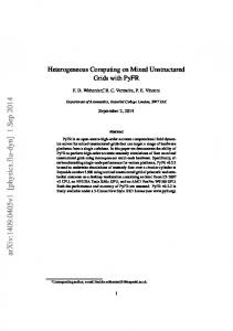
For each case (linear, quadratic and cubic) and each mesh (labeled by element size h) we exercise various Runge-Kutta integrators and interpolation schemes and we vary the relative spatial step size ∆s/h. Fig. 2 is a contour plot of transit time error tracking with the Euler (1st order) method and using linear interpolation on a mesh of linear element shapes and basis functions. The error with quadratic interpolation is identical. Contours of run time on a 500 MHz PC are also shown. To make the step-induced error small compared to the grid-induced error, many steps per element are required as one refines the mesh. Fig. 3 is a similar plot for tracking with the improved
10−2
10−1
relative spatial step size ∆s/h
100
Figure 3: Transit time error (solid) and run time (dashed) for tracking with the modified Euler method and quadratic interpolation. Euler (2nd order) method. Only a few steps per element are needed in order to reduce the step-induced tracking error to a fraction of the grid induced error. Note that we expect these two plots to bound the transit time error from a Boris-type pusher on an unstructured grid which doesn’t stop and restart at element boundaries. At sufficiently large step size a Boris push will have 2nd order convergence, but at smaller step sizes it will have only 1st order convergence due to the discontinuities in the electric field. Unfortunately, this 1st order convergence will appear when the step-induced errors are approximately an order of magnitude larger than the grid-induced errors. In contrast to such a Boris-type pusher, the novel particle tracking algorithm maintains its convergence rate even when the step size is small. Fig. 4 shows that, even at one step per element, the stepinduced tracking error is negligible compared to the gridinduced tracking error when using the classical 4th order Runge-Kutta method with cubic interpolation on a linear mesh with a linear basis. Which tracker and what step size should one use? If the mesh can be easily coarsened or refined then the element and step sizes might be chosen to provide the greatest accuracy in the least time. If the mesh is fixed, then one might choose the step size small enough to make the step-induced error a modest fraction of the grid-induced error, but not much smaller. Looking at run time vs accuracy on a linear mesh with a linear basis, the best choice is the classical 4th order Runge-Kutta method with quadratic interpolation at ∼2 steps per element. The cubic interpolation scheme suffers from a robust but slow bisection polynomial root solver. We plan to improve this root solver and reassess the run time with cubic interpolation.
3058
Proceedings of the 2001 Particle Accelerator Conference, Chicago
10
0
10
s
3
s
element size h
0.1
10
10−2
10−1
relative spatial step size ∆s/h
100
10−5
10 4 s
0.05
10−6
10−3
Figure 4: Transit time error (solid) and run time (dashed) for tracking with the classical 4th order Runge-Kutta method and cubic interpolation.
Fig. 5 shows the behavior of the classical 4th order Runge-Kutta method with cubic interpolation on a cubic mesh with a cubic basis. Some error cancellation is evident in the shape of the contour lines. We qualitatively remove such cancellations in our assessments of accuracy vs run time. The classical 4th order Runge-Kutta is the best choice for accuracy vs time for the cubic case. Use either quadratic interpolation at 10–20 steps per element or cubic interpolation at ∼10 steps per element. We’ve found that the 1st and 2nd order Runge-Kutta methods are clearly inadequate for the cubic mesh/basis because particle tracking consumes orders of magnitude more time than the field solver in order to reduce the step-induced tracking errors to the level of the grid-induced tracking errors.
10−2
relative spatial step size ∆s/h
10−2
struct-li
STRUCTURED GRID COMPARISON
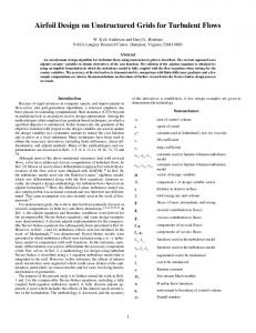
We ran the same test model using the MICHELLE code’s Boris pusher on a conformal structured grid of linear hexahedral elements. There are no transverse position or momentum errors in this case. The transit time and momentum at the discretized outer cylinder surface was linearly interpolated from the last step of the trajectory. The gridinduced transit time error for the conformal structured grid is much smaller than a comparable size unstructured grid of linear tetrahedral elements. Fig. 6 compares accuracy vs run time. The linear structured grid with a Boris pusher is 10–20 times faster than the linear unstructured grid with the novel particle tracking algorithm. The scaling with time is similar. The quadratic and cubic unstructured grids are superior to the linear structured grid.
unstru
100
ct-line
near-bo
ris
10−3
ar
unstru
ct-qu
−4
adrati
unst
10
ruct-
c
cubi
c
−5
10
1
3
10
30
100
300
1000
CPU time (sec) Figure 6: Transit time error vs run time.
6 5
10−1
Figure 5: Transit time error (solid) and run time (dashed) for tracking with the classical 4th order Runge-Kutta method and cubic interpolation on a cubic mesh with a cubic basis.
transit time error
element size h
10−4
10−2 10 3 s
10−3
s
0.2
10 2 s
0.05
2
s
0.1
10−1
10 1 s
10
1
0.2
CONCLUSION
We’ve demonstrated the capabilities of the novel particle tracking algorithm on a simple test problem. The modest convergence of the transverse position on a linear mesh with a linear basis is a concern, but the convergence with a quadratic or cubic mesh/basis is very good. Much work remains, however, before we are confident that we can accurately model a device as complicated as a gridded gun. For example, performance in the presence of space charge needs to be studied. Also, the accuracy of the finite element solution for the electric potential in the presence of sharp corners and edges needs to be evaluated, and the expected degradation in accuracy needs to be mitigated.
3059