15th Int Symp on Applications of Laser Techniques to Fluid Mechanics Lisbon, Portugal, 05-08 July, 2010
Particles Depth Detection using In-Line Digital Holography Configuration Sanjeeb Prasad Panday1, Kazuo Ohmi2, Kazuo Nose2 1: Department of Information Systems Engineering, Graduate School of Osaka Sangyo University, Japan,
[email protected] 2: Information Systems Engineering, Osaka Sangyo University, Japan,
[email protected];
[email protected]
Abstract Digital holography (DH) is the direct recording of the Fresnel or Fourier holograms using a CCD or CMOS camera and is considered as an alternative to the optical holography which uses a film or a plate involving wet-chemical or other processes. However, the poor pixel resolution of CCD or CMOS cameras as compared to that of holographic films gives poor depth resolution for images which in turn severely undermines the usefulness of digital holography in densely populated particle fields. The authors in this paper present a technique of depth measurement for the detection of the depth of small tracer particles distributed in 3-D space. This technique is based on in-line holography and the depth of the particles is measured using the numerically reconstructed images obtained from the convolution based Fresnel Reconstruction formula. The particle depth is measured by determining the distribution of light intensity within a proper rectangular sampling window around the test particle. The sample median, mean and minimum value approach is employed as an averaging technique for the light intensity measured at all pixels within that rectangular sampling window and the position on the z-axis where all these values are minimum is regarded as the depth of that particular test particle. The present method is successfully applied to the hologram pattern with overlapping interference fringes which signifies the applicability of the present method to the flow measurements.
1. Introduction Holography is regarded as a powerful tool for the recording of a 3-D object and the measurement of its shape, displacement, deformation and vibration in various fields of engineering. Holography is a method of recording the light reflected or transmitted from a projected object to a photo-plate in the form of interference pattern. For recording, an object beam and a reference beam are required, and as the result of combining two beams, an interference pattern is made. In the past, the interference patterns were recorded on a film plate. Recent advances in charge-coupled device (CCD) and computer technology have permitted replacing holographic films with CCD arrays and optical reconstruction with computer-driven numerical reconstruction. The use of holography for the diagnostics of small particles can be traced back to late 1960’s (Trolinger et al. 1969). Although powerful, the conventional procedure of holography, which includes film-based recording, wet chemical processing and optical reconstruction, has severely restricted the user friendliness of the holographic imaging technique (Pu and Meng 2000; Bishop et al. 2001; McIntyre et al. 2003). In this regard, digital holography (Yamaguchi and Zhang 1997; Nilsson and Carlsson 1998; Dubois et al. 1999; Yu and Cai 2001) which records holograms directly to digital media such as CCD or CMOS sensors and reconstructs the objects numerically looks very promising. Digital holography is referred to as the technique that uses a CCD or CMOS camera to record holographic patterns and performs the reconstruction numerically using a computer. The numerical hologram reconstruction was initiated in the early 1980s (Yaroslavskii and Merzlyakov 1980). Onural and Scott (1987) further improved this reconstruction algorithm and applied it to particle measurements. However, the entire recording and reconstruction of hologram has not been digitalized yet. Schnars and Jüptner (1994) were the first to propose the technique of digital holography for 3-D objects of large volume. They reconstructed the image on a digital computer -1-
15th Int Symp on Applications of Laser Techniques to Fluid Mechanics Lisbon, Portugal, 05-08 July, 2010
from a hologram pattern observed with a CCD camera and examined the quality of reconstructed images as well as the procedure of fringe analysis for the digitized hologram patterns in detail to show the excellent images obtained by digital image reconstruction using a cubic die. This method now enables digital recording and processing of holograms, without any photographic recording as intermediate step. However, the poor pixel resolution of CCD or CMOS cameras as compared to that of holographic films severely undermines the usefulness of digital holography in densely populated particle fields. In this regard, the main objectives of this paper are to demonstrate the numerical reconstruction process of particles holograms in different planes based on the Fresnel Convolution Scheme (Schnars and Jüptner 2002) and to apply the technique of digital image reconstruction to particle depth measurement. The authors have proposed a holographic method for the depth measurement of small particles distributed in 3-D space and have also examined the measurement accuracy of the method. This method based on in-line digital holography has not only the advantage of easy camera setting in experiments but it also gets rid off troublesome process of particle identification afterwards, when compared with a stereoscopic method that is often used for 3D particle tracking velocimetry (3D-PTV) in fluid engineering.
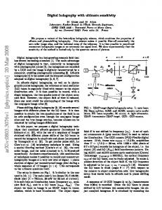
2. Digital holography fundamentals Digital holography is a technique of holography in which hologram patterns are obtained with an electronic camera, and its image reconstruction is numerically carried out on a digital computer. In the same manner as conventional holography, the digital holography also consists of two stages namely recording and reconstruction stages but since the development of a hologram is not required in digital holography, the procedure is suitable for on-line measurement. Fig. 1 shows hologram recording and image reconstruction in digital holography for a small particle. During the recording stage, an expanded laser beam (a plane reference wave) illuminates the object in the object plane. Then the interference pattern obtained from the interference of this expanded laser beam and the light diffracted from the object, a small particle in this case, is recorded with a CCD or CMOS camera in the hologram plane as shown in Fig. 1(a). In the reconstruction stage of the conventional holography, the same plane reference wave illuminates the recorded hologram and the reconstructed image of the object can be seen at the same distance as between the object and the hologram in the recording phase whereas in the case of the digital holography, this is performed numerically in the computer. Fig 1(b) shows the reconstruction stage of the both holography techniques.
d
Plane Wave
Object Plane
Hologram
(a) Hologram recording -2-
15th Int Symp on Applications of Laser Techniques to Fluid Mechanics Lisbon, Portugal, 05-08 July, 2010
z
Hologram
d
Image Plane
Hologram
Plane Wave
(b) Hologram reconstruction Fig. 1 Recording and reconstruction stages of digital holography
2.1 Numerical reconstruction In this research, the digitally recorded hologram is numerically reconstructed in the computer by using the convolution (CV) approach (Schnars and Jüptner 2002). In this approach of reconstruction, the reconstruction wave is defined as the convolution of the product of the reference wave and the digital hologram function with the impulse response function of coherent optical system. Mathematically, the reconstructed wave can be expressed as:
[(
)
Γ (ξ ,η ) = R * (k , l )h(k , l ) ⊗ g (k , l )
]
(1)
where ⊗ indicates a two-dimensional convolution, R*(k, l) is the conjugate of the plane reference wave R(k, l), h(k, l) is the hologram function and g(k, l) is the numerical impulse response function of the coherent optical system. Application of the convolution theorem to equation (1) yields:
{(
)
}
Γ (ξ ,η ) = ℑ−1 ℑ h ⋅ R ∗ • ℑ ( g )
(2)
To save the computation time for the calculation of one Fourier transform, the Fourier transform of g is analytically expressed in equation (3). 2 2 N 2 ∆x 2 N 2 ∆y 2 2 2 λ m + λ n + 2πd 2dλ 2dλ ℑ ( g ) = G (n , m) = exp − i 1− − λ N 2 ∆x 2 N 2 ∆y 2
(3)
Equation (2) shows that the reconstructed object wave can be calculated first by Fourier transforming the product of the digital hologram and the reference wave. This is then followed by -3-
15th Int Symp on Applications of Laser Techniques to Fluid Mechanics Lisbon, Portugal, 05-08 July, 2010
multiplying with the Fourier transform of the numerical impulse response function of coherent optical system (g) and taking an inverse Fourier transform of this whole product. Substituting equation (3) into equation (2), we get:
{(
) }
Γ (ξ ,η ) = ℑ−1 ℑ h ⋅ R∗ • G
(4)
This equation (4) is implemented by the authors in this communication for the reconstruction of the recorded hologram. The intensity of the reconstructed hologram is determined by calculating the square of the magnitude of Γ (ξ, η) as given by equation (5). I (ξ ,η ) = Γ(ξ ,η )
2
(5)
2.2 Detection of the depth of a particle In the particle tracking based method, particle positions provide measuring positions in 3-D space, so the positions must be accurately measured prior to velocity measurement. If a hologram is recorded by illuminating a particle from left to right by an extended laser beam as shown in Fig. 1(a) then the particle image observed on a hologram is its shade and the light intensity on the shade is lower than that of background (Murata and Yasuda 2000). Therefore, on the line passing through the center of axisymmetric fringes and perpendicular to the hologram (z-axis in Fig. 1(b)), the light intensity becomes minimum at the particle depth. So, the particle depth can be measured by detecting the position on the z-axis where the light intensity is minimum. The authors have used the same principle to detect the depth of particles from the reconstructed hologram in this paper. In order to reduce the computing time required, the center of the particle is measured using image processing application software and then the distribution of light intensity is determined within a proper rectangular sampling window which is chosen from the center of that particle. The sample median, mean and minimum intensity value approach is employed as an averaging technique for the light intensity measured at all pixels within that rectangular sampling window. Then the graph is plotted between these values and the distance along the z-axis. The position on the z-axis (zcoordinate) where all these three intensity values of the light intensity (mean, median, minimum intensity) are minimum, gives the depth of the particle.
3. Test Results CMOS
Laser
Filter
To computer Particle field
Beam expander
Hologram (sensor plane)
Fig. 2 Experimental set-up for recording hologram Various optical geometries have been proposed till now for particle analysis using the digital holography. But the simplest and most common optical system for particle analysis is by using the -4-
15th Int Symp on Applications of Laser Techniques to Fluid Mechanics Lisbon, Portugal, 05-08 July, 2010
collimated laser beam. In this research, a collimated laser beam is expanded and then used to shine the particle field distribution as shown in Fig. 2. The experiment is carried out using this in-line holography set-up. The digital hologram is recorded by using the small water tank of size 156X81X16 mm3 which is filled with water and randomly distributed micro Orgasol particles of sizes ~60 µm. He-Ne laser beam having wavelength of 632.8 mm is used to illuminate the water tank for hologram recording. Digital hologram of the particles thus obtained was directly recorded by an 8-bit CMOS camera (Silicon Video 9M001) with 512 X 512 pixels of size 5.2 µm. This CMOS camera is kept at a distance of 45 mm from the water tank. Fig. 3 depicts a typical hologram of micro-particles recorded using the in-line holography set-up in Fig. 2.
Fig. 3 A recorded typical hologram of particles Test Particle X In focus particle Out of focus particle
(a) Intensity image at z = 46 mm
Test Particle Y
(b) Intensity image at z = 50 mm
Fig. 4 Reconstructed images at different z distances
-5-
15th Int Symp on Applications of Laser Techniques to Fluid Mechanics Lisbon, Portugal, 05-08 July, 2010
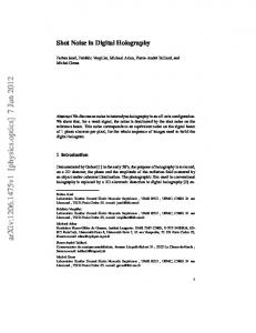
In this communication, the authors have chosen the convolution approach for reconstruction of the hologram as in this case the pixel size of the reconstructed image is independent of the holographic arrangement parameters and is equal to the size of CCD or CMOS pixel. However, one serious drawback of the convolution method is that it suffers from the interference called wraparound error. In order to avoid this error, the authors have stretched the size of the recorded hologram artificially from 512 X 512 to 1024 X 1024 by padding zeros around the original image before applying the reconstruction algorithm. Though this increases space and time complexity, the results are free from wrap-around errors. Equations (3), (4) and (5) are used for the numerical reconstruction of hologram. The intensity images of the numerically reconstructed holograms at distances z = 46mm and z = 50 mm are shown in Fig. 4(a) and Fig. 4(b) respectively. In both these images, the in-focus particles appear as sharp black dots while the out-of-focus particles appear as hollow light concentric circles. It can also be noticed that the particles which appear as focused at certain distance are defocused and disappeared when the reconstruction distance is changed. This signifies the possibility of locating each particle individually at different depths using a single recorded hologram. As already discussed in the Section 2.2, to detect the depth of the test particle “X” shown in Fig. 4(a) at first 4X4 rectangular sampling window is chosen such that the test particle is at the center of this sampling window. The sample median, mean and minimum intensity value is then calculated for all the pixels within the same rectangular sampling window. Now, the graph showing the variation of these values with respect to the distances along the z-axis is plotted. The depth of the particle is then given by that z-coordinate at which all these three values of the light intensity become minimum. Fig. 5 shows the graph which shows the variation of the light intensity distribution (in terms of median, mean and minimum) along the z-axis and Table 1 gives the data for the test particle “X”. From both the graph and the table, it can be clearly observed that test particle “X” is located at the distance 50 mm from the camera as all the intensity values are minimum at this distance. This result is also verified from the numerically reconstructed images at different z distances. The same process is repeated to find the depths of other remaining particles. 120 Median Mean Minimum 100
Intensity
80
60
40
20
0 45
46
47
48
49
50
51
52
53
54
55
56
57
58
59
60
61
Z (Distance)
Fig. 5 Light Intensity distribution around the test particle “X” along z-axis -6-
15th Int Symp on Applications of Laser Techniques to Fluid Mechanics Lisbon, Portugal, 05-08 July, 2010
Table 1 Light Intensity distribution data for particle “X”
z (Distances)
Median Mean
Minimum
45
81
84.75309
57
46
71
71.50617
30
47
53
56.74074
22
48
48
46.76543
12
49
33
44.8642
7
50
32
43.09877
0
51
42
45.88889
4
52
41
45.75309
19
53
50
54.54321
28
54
68
68.8642
37
55
74
75.58025
51
56
84
86.19753
65
57
90
90.51852
66
58
92
93.66667
73
59
95
96.08642
76
60
98
96.40741
71
61
94
95
73
80 Median Mean Minimum
70
60
Intensity
50
40
30
20
10
0 45
46
47
48
49
50
51
52
53
54
55
56
57
58
59
60
61
Z (Distance)
Fig. 6 Light Intensity distribution graph and data around the test particle “Y” along z-axis -7-
15th Int Symp on Applications of Laser Techniques to Fluid Mechanics Lisbon, Portugal, 05-08 July, 2010
Further, in the similar way as done for test particle “X”, it can be concluded from Fig. 6 that the another test particle “Y” is located at the distance 48 mm from the camera as all the intensity values are minimum at this distance. This result is also verified from the numerically reconstructed images at different z distances. Thus, it can be concluded that the present method is useful for the depth measurement of small particles distributed in 3-D space. Once the spatial (x,y,z) coordinates of the particles have been identified in the above mentioned way then any particle tracking algorithm can be used to successfully track the particles.
4. Conclusions In this paper, the method for numerically reconstructing the hologram using convolution method and then the technique to detect the depths of small particles present in the numerically reconstructed holograms is presented. From the test results, it can be concluded that the present method is useful for the depth measurement of small particles distributed in 3-D space. In the current method, the sampling window size is chosen by hit and trial method. If the window size is too large or too small, there may be an error in the depth of the particles. Thus, care should be chosen while selecting the size of the sampling window. It is expected that the better results can be obtained if higher spatial resolution CCD or CMOS camera is used. Further, the current technique is tested only with few numbers of particles. Hence, the authors will make further efforts to improve this algorithm so that it can be used to detect and track the higher number of particles in their future work.
References Bishop AI, Littleton BN, Mclntyre TJ, Rubinstein-Dunlop H (2001) Near-resonant holographic interferometry of hypersonic flow. Shock Waves, 11:23–29 Dubois F, Joannes L, Legros J (1999) Improved three-dimensional imaging with a digital holography microscope with a source of partial spatial coherence. Applied Optics, 38:7085-7094 McIntyre TJ, Bishop AI, Eichmann TN, Rubinsztein-Dunlop H (2003) Enhanced flow visualization using near-resonant holographic interferometry. Applied Optics, 42:4445–4451 Murata S, Yasuda N (2000) Potential of digital holography in particle measurement. Optics & Laser Technology, 32:567-574 Nilsson B, Carlsson TE (1998) Direct three-dimensional shape measurement by digital light-in-flight holography. Applied Optics, 37:7954-7959 Onural L, Scott PD (1987) Digital decoding of in-line holograms. Optics Engineering, 26:1124-1132 Pu Y, Meng H (2000) An advanced off-axis holographic particle image velocimetry _HPIV_ system. Experiments in Fluids, 29:184–197 Schnars U, Jüptner W (1994) Direct recording of holograms by a CCD-target and numerical reconstruction. Applied Optics, 33:179-181 Schnars U, Jüptner W (2002) Digital recording and numerical reconstruction of holograms. Measurement Science and Technology, 13:R85–R101 Trolinger JD, Beltz RA, Farmer WM (1969) Holographic techniques for the study of dynamic particle fields. Applied Optics, 8:957-961 Yamaguchi, Zhang T (1997) Phase-shifting digital holography. Optics Letter, 22:1268-1270 Yaroslavski LP, Merzlyakov NS (1980) Methods of Digital Holography. Consultants Bureau, New York Yu L, Cai L (2001) Iterative algorithm with a constraint condition for numerical reconstruction of a threedimensional object from its hologram. Journal of the Optical Society of America A, 18:1033-1045
-8-