Partition function of nearest neighbour Ising models: Some new insights
Recommend Documents
(2) where λ1 and λ2 denote the eigenvalues: /. 2. 4 /. 1 cosh sinh. J kT. J kT. H. H e e. kT. kT λ. â. â¡. â¤. â ..... John Wiley) 1st edn. 5. Onsager L 1944 Phys. Rev.
105â113. c Indian Academy of Sciences. Partition function of the two-dimensional nearest neighbour Ising models for finite lattices in a non-zero magnetic field.
the values of Yang and Lee while the corresponding 'dimensionless' magnetic ...... Chamberlin, R.V. Mean-field model for the critical behaviour of ferromagnets.
Fig.1: The variation of the partition function with the nearest neighbour interaction energies for various values of N. Lines denote the estimates arising from the ...
and is applied in diverse contexts: the study of critical behaviour of ... In view of its equivalence with binary alloys and lattice gas .... Harvard University. Press ...
Aug 16, 2012 - integer paramagnetic phases can be found at zero temperature. ...... However, the absolute values predicted for the ground state energy, and spinodal ..... regimes of ground state energy zero become rarer, and unattainable.
be purchased through online sources. The nearest neighbour ... map, as in this case, the researcher must ensure there is
the nni-distance between two arbitrary n-node trees from 4nlog n 2] to nlog n. ... the subtrees to create either of the trees on the right, with associated partitions.
vised NNDM, two instances that belong to different classes will be pushed apart from each other. .... class. The illustration of the distance loss function applied in.
Dec 27, 2013 - arXiv:1312.7289v1 [math-ph] 27 Dec 2013. GRAPH ...... planarity criterion [27], starting from the following constatation: Proposition 3.11.
CORRELATION OF NEAREST NEIGHBOUR. DISTANCE AND BONDING PARAMETERS. OF EXAFS OF SOME Mn AND Co SYSTEMS. V.K. SINGH AND A.R. ...
Evaluating the Performance of Nearest Neighbour Algorithms when Forecasting US Industry Returns. 1. C. S. Pedersen. 2. S. E. Satchell. 3. Abstract. Using both ...
Apr 4, 2016 - r=k(G) e(G). â s=0 zrsqrvs. (1.5) where k(Gâ²) denotes the number of ..... For the graphs Lm with odd m, Ï(Lm) = 5, so that Z(G, 4,v) contains at ...
rough ownership function (FRNN-O) approach. By contrast to the latter, our method uses the nearest neighbours to construct lower and upper approximations of ...
Abstract. A new fuzzy-rough nearest neighbour (FRNN) classification algorithm is presented in this paper, as an alternative to Sarkar's fuzzy- rough ownership ...
the measurement system because the accuracy of the ... the representative is the gray-based assays; the other one is the SUSAN ... This algorithm can do the dilation operation based on the ... rated, extract image outlines, and then make polygon fitt
ABSTRACT. Nearest Neighbour algorithms for pattern recognition have been widely studied. It is now well-established that they offer a quick and reliable ...
We propose a modified nearest neighbour algorithm for ..... The reader can verify that the maximum .... http://www.cs.waikato.ac.nz/ml/weka/index datasets. html ...
Nearest neighbour. Classification. Fuzzy-rough sets have enjoyed much attention in recent years as an effective way in which to extend rough set theory such ...
Dec 25, 2006 - Nearest neighbour model for prediction of weather in terms of snow day/no .... Ten nearest days, prior situations to the nearest situa- tions, next ...
In this example, researchers have mapped the land use of each building in a 200m by 200m plot in a town centre, using a
Visualization. Using. Arbitrary Triangulations. Frank Weller and Robert Mencl ..... 7] Pascal Fua and Peter T. Sander. Reconstructing surfaces from un- structured ...
NEAREST NEIGHBOUR CLASSIFICATION ON LASER POINT CLOUDS. TO GAIN OBJECT STRUCTURES FROM BUILDINGS. B. Jutzi a, H. Gross b a. Institute ...
We introduce a novel algorithm for solving the nearest neighbour problem when the query points are known in advance, which is based on Fortune's plane ...
Partition function of nearest neighbour Ising models: Some new insights
Abstract. The partition function for one-dimensional nearest neighbour Ising models is estimated by summing all the energy terms in the Hamiltonian for N sites.
Partition function of nearest neighbour Ising models: Some new insights† G NANDHINI and M V SANGARANARAYANAN* Department of Chemistry, Indian Institute of Technology Madras, Chennai 600 036 e-mail: [email protected] Abstract. The partition function for one-dimensional nearest neighbour Ising models is estimated by summing all the energy terms in the Hamiltonian for N sites. The algebraic expression for the partition function is then employed to deduce the eigenvalues of the basic 2 × 2 matrix and the corresponding Hermitian Toeplitz matrix is derived using the Discrete Fourier Transform. A new recurrence relation pertaining to the partition function for two-dimensional Ising models in zero magnetic field is also proposed. Keywords. Ising model; partition function, Toeplitz matrix; recurrence relation; Discrete Fourier Transform.
1.
Introduction
The analysis of nearest neighbour Ising models plays a crucial role in diverse contexts such as order– disorder transitions,1 adsorption at electrochemical interfaces,2 protein folding,3 etc. While the formulation of the partition function pertaining to onedimensional nearest neighbour Ising models is pedagogical and straight-forward,4 the same is not true for the two-dimensional Ising models. The celebrated solution of Onsager5 for the two-dimensional Ising model at H = 0 led to the detailed analysis of critical temperatures and critical exponents. However, several approximate treatments for the analysis of two-dimensional Ising models employing Bragg– Williams approximation,6 Bethe ansatz,7 series expansions,8 etc. are available in addition to the Monte Carlo simulations.9 A significant accomplishment regarding the exact solution of the two-dimensional Ising models consists in the application of the renormalization group techniques10 for the study of critical phenomena. Nevertheless, the exact partition function for the two-dimensional Ising model in the presence of the external magnetic field (H ≠ 0) leading to the critical properties is still lacking. A plausible strategy to obtain new insights regarding the analysis of two-dimensional Ising models is to formulate new procedures even for one-dimensional Ising models in anticipation that this new methodo†
Dedicated to the memory of the late Professor S K Rangarajan *For correspondence
logy may lead to the exact solution of the twodimensional Ising models in presence of an external magnetic field. It is of interest to point out here that the partition function for one-dimensional nearest neighbour Ising models for N sites is customarily derived by deducing the eigenvalues of a 2 × 2 Matrix and subsequently generalized to the thermodynamic limit N → ∞. The objectives of the present Communication are (i) to report the partition function of one-dimensional nearest neighbour Ising models by summation of all the energy terms in the Hamiltonian for small values of N; (ii) to re-construct the matrix from the known eigenvalues and (iii) to postulate a recurrence relation between the partition function for N and 2N sites. 2. Partition function of one-dimensional nearest neighbour Ising models The Hamiltonian for the one-dimensional Ising model is N
N
i =1
i =1
H T = − J ∑ σ iσ i +1 − H ∑ σ i ,
(1)
where J denotes the nearest neighbour interaction energy and H denotes the external magnetic field. It is customary to construct a basic 2 × 2 matrix consisting of the matrix elements which takes into account, various arrangements of the spin variables 595
596
G Nandhini and M V Sangaranarayanan
+(6e 2 J/kT + 12e −2 J/kT + 2e −6 J/kT ),
(+1, +1; –1, +1; +1, –1 and –1, –1). The canonical partition function then is deduced as4 QN = (λ1N + λ2N ),
(2)
⎛ 8H Q8 = 2e8 J/kT cosh ⎜ ⎝ kT
where λ1 and λ2 denote the eigenvalues:
⎛ e1/kT ( J + H ) Q = ⎜ − J/kT ⎝ e
(4)
One of the two eigenvalues being the most dominant, estimation of the partition function in the thermodynamic limit and extraction of the internal energy, specific heat, etc. becomes straight-forward. 2.1 Partition function from the summation of the energy terms In stead of the above method involving the formulation of the matrix and computing the partition function from the eigenvalues, we investigate here, the consequences of summation of the energy terms directly. The partition function obtained by summing the energy terms for different values of N (3 and 6; 4 and 8) are as follows: ⎛ 3H Q3 = 2e3 J/kT cosh ⎜ ⎝ kT
⎡ ⎤ ⎛H ⎞ ⎛H ⎞ λ1 = e J/kT ⎢cosh ⎜ ⎟ + sinh 2 ⎜ ⎟ + e−4 J/kT ⎥ ⎝ kT ⎠ ⎝ kT ⎠ ⎥⎦ ⎣⎢ ⎡ ⎛H ⎞ 2⎛ H ⎞ −4 J/ kT λ2 = e J/kT ⎢cosh ⎜ ⎟ − sinh ⎜ ⎟+e ⎝ kT ⎠ ⎝ kT ⎠ ⎢⎣ which arise from the matrix
(7)
+(8e 4 J/kT + 36 + 24e−4 J/kT + 2e −8 J/kT ) .
(8)
Equations (5) to (8) were deduced by listing all the energy terms of (2) using MS EXCEL (2N terms arise for a lattice of N sites). Although the procedure is valid for any value of N, we restricted the enumeration to a small number of sites so as to avoid algebraic complexity as well as for obtaining a recurrence relation for the partition function. 2.2
Eigenvalues from the partition function
As an illustration, consider the partition function obtained by summation of the energy terms in the Hamiltonian (1) for N = 4: ⎛ 4H ⎞ ⎛ 2H ⎞ −4 J/kT Q4 = 2e 4 J/kT cosh ⎜ ) ⎟ + 8cosh ⎜ ⎟ + (4 + 2e ⎝ kT ⎠ ⎝ kT ⎠
Partition function of nearest neighbour Ising models
As can be seen from (2), Q4 can also be represented as Q4 = (λ14 + λ24 ),
(10)
where λ1 and λ2 denote the eigenvalues of the matrix corresponding to the one-dimensional Ising model. A comparison of (9) and (10) leads to the eigenvalues as given by (3). 2.3
In view of the availability of convenient expressions for Q, it is imperative to verify whether there exists any pattern among the partition function for different values of N. Using well-known identities involving trigonometric functions,11 it can be shown that ⎛ 2J ⎞ Q2 N = QN2 − 2 N +1 sinh N ⎜ ⎟, ⎝ kT ⎠
(11)
for all values of N. The above eqn thus enables predicting the partition function for a lattice of 2N sites from the value pertaining to N sites.
In the present approach, while the partition function and the eigenvalues have been obtained, the underlying matrix has not yet been derived. Obviously, the matrix is not unique for a given eigenspectrum; however, the construction of such matrices may provide an insight into the solution of higher dimensional Ising models. To obtain the matrix, we apply a procedure demonstrated in the context of signal processing12 employing the Discrete Fourier Transform. For a given set of eigenvalues (λ0, λ1, …, λn–1), the parameters qk are defined as:
2.4 Inverse problem of constructing the matrix from the eigenvalues
qk =
while the desired matrix constructed from the above is as follows,12
(12)
(15)
The associated matrix [q] consisting of elements qk is given below: (cf. Appendix A):
It is of interest to note that the above Hermitian Toeplitz matrix is entirely different from the hith-
598
G Nandhini and M V Sangaranarayanan
erto-known matrix (4) for one-dimensional nearest neighbour Ising models.
and k1 =
3. Two-dimensional nearest neighbour Ising models It will be of interest to verify whether this methodology will be applicable to two-dimensional Ising model in presence of the external magnetic field. The summation of energy terms for two-dimensional Ising model for H ≠ 0 has earlier been carried out by us13 and the formulation of the matrix using the Discrete Fourier Transform is under progress. However, here we make use of the Onsager’s exact solution for H = 0 and demonstrate the validity of the recurrence relation (11) for two-dimensions also. Such recurrence relations can enable extrapolation of Monte Carlo and molecular dynamics simulation results for larger system sizes. The canonical partition function for H = 0 arising from Onsager’s exact solution is given by5 ⎡ ⎛ 2J QH=0 = ⎢ 2cosh ⎜ ⎝ kT ⎣
(17)
Employing the above equations, it is possible to estimate Q for different values of N. Since our essential focus has been on the square lattice, we first substitute N = 16 in (11) and calculate Q for N = 32; subsequently, the value of Q for N = 64 is evaluated from (11). This estimated value is compared with Q values arising from (16) for N = 64 (figure 1). As can be seen from figure 1, the agreement is entirely convincing, suggesting that the recurrence relation (11) is valid for two-dimensional nearest neighbour Ising model too, when H = 0. It is interesting to note that the values for N = 16 was employed as the input to predict the values for N = 64. 4.
Summary
N
⎞ I⎤ ⎟e ⎥ , ⎠ ⎦
(16)
where π
I=
2sinh(2 J/kT ) . cosh 2 (2 J/kT )
1 1 log(1 + 1 − k12 sin 2 φ )dφ 2π ∫0 2
An alternate method for estimating the partition function of one-dimensional nearest neighbour Ising model is proposed. A new recurrence relation is proposed for the partition function for N sites. A Hermitian Toeplitz matrix is constructed from the eigenvalues, using the Discrete Fourier Transformation. The significance of this method for twodimensional Ising models when H = 0 is indicated. Acknowledgement This work was supported by the Department of Science and Technology (DST), Government of India, New Delhi. Appendix A
Figure 1. The comparison of the partition function values from Onsager’s exact solution (16) with the values predicted by the recurrence relation (11) The points denote the values from (11) for Q64 employing the values of Q16 from Onsager’s exact solution (16) while the line is the predicted values from (16) employing N = 64.
In this Appendix, the steps leading to the construction of the matrix (14) from the eigenvalues spectrum is indicated. The analysis is identical with that of12 employed in the context of signal processing. A negacyclic real symmetric matrix of order n can be obtained from a set of n distinct eigenvalues by use of the inverse DFT, qk =
π 1 n −1 λi cos (2i + 1)k , k = 0,1, ..., n − 1. ∑ n i =0 m
Partition function of nearest neighbour Ising models
As an illustration, for an eigen spectrum consisting of 3 eigenvalues, n = 3 and hence m = 2n = 6, a 6 × 6 matrix is first constructed. ⎡ q0 ⎢q ⎢ 1 ⎢ q2 [ qex ] = ⎢ ⎢ 0 ⎢ − q2 ⎢ ⎢⎣ −q1
q1
q2
0
− q2
q0 q1
q1 q0
q2 q1
0 q2
q2
q1
q0
q1
0 − q2
q2 0
q1 q2
q0 q1
− q1 ⎤ − q2 ⎥⎥ 0 ⎥ ⎥. q2 ⎥ q1 ⎥ ⎥ q0 ⎥⎦
The above matrix can be re-written in the form ⎡[ A] −[ B ]⎤ ⎢[ B ] [ A] ⎥ ⎣ ⎦
where ⎡ q0 ⎢ [ A] = ⎢ q1 ⎢⎣q2
q1 q0 q1
q2 ⎤ ⎡ 0 ⎥ q1 ⎥ , [ B] = ⎢⎢ −q2 ⎢⎣ −q1 q0 ⎥⎦
q2 0 − q2
q1 ⎤ q2 ⎥⎥ . 0 ⎥⎦
If we assume the matrix elements of A as a11, a12, a13, etc. and that of the matrix B as b11, b12, b13, b21, b22, etc. it follows that a11 = q0, a12 = q1, …, a33 = q0 and b11 = 0, b12 = q2, …, b33 = 0, the desired matrix C with the elements c11, c12, etc. are obtained as c11 = a11 – ib11, c12 = a12 – ib12, …, c33 = a33 – ib33, yielding
⎡ q0 C = ⎢⎢q1 + iq2 ⎢⎣q2 + iq1
q1 − iq2 q0 q1 + iq2
599
q2 − iq1 ⎤ q1 − iq2 ⎥⎥ . q0 ⎥⎦
where i = (–1)1/2. This procedure was employed for deducing the matrix (15) pertaining to the onedimensional Ising model. References 1. Bonaccorsi E, Merlino S, Pasero M and Macedonio G 2001 Phys. Chem. Miner. 28 509 2. Basha C A and Sangaranarayanan M V 1989 J. Elec. Anal. Chem. 261 431 3. Lenz P, Zagrovic B, Shapiro J and Pande V S 2004 J. Chem. Phys. 120 6769 4. Huang K 1963 Statistical mechanics (New York: John Wiley) 1st edn 5. Onsager L 1944 Phys. Rev. 65 117 6. Bragg W L and Williams E J 1934 Proc. Roy. Soc (London) A145 699 7. Bethe H A 1935 Proc. Roy. Soc. (London) A150 552 8. Domb C, In Domb C and Green M S (eds) 1974 Phase transitions and critical phenomena (London: Academic Press) vol 3, pp. 357–484 9. David P, Landau and Kurt Binder 2000 A guide to Monte Carlo simulations in statistical physics (Cambridge University Press) p. 71 10. Wilson K G 1971 Phys. Rev. B4 3174 11. Gradshteyn I S and Ryzhik I M 1996 Table of integrals, series and products (Academic Press) p. 31 12. Noor F and Morgera S D 1992 IEEE Trans. Signal Process. 40 2093 13. Nandhini G and Sangaranarayanan M V archives: http://uk.arxiv.org/ftp/arxiv/papers/0710/0710.3688.pdf