Graph theory and Pfaffian representations of Ising partition function

GRAPH THEORY AND PFAFFIAN REPRESENTATIONS OF ISING PARTITION FUNCTION.

arXiv:1312.7289v1 [math-ph] 27 Dec 2013

THIERRY GOBRON Abstract. A well known theorem due to Kasteleyn states that the partition function of an Ising model on an arbitrary planar graph can be represented as the Pfaffian of a skewsymmetric matrix associated to the graph. This results both embodies the free fermionic nature of any planar Ising model and eventually gives an effective way of computing its partition functions in closed form. An extension of this result to non planar models expresses the partition function as a sum of Pfaffians which number is related to the genus of the oriented surface on which the graph can be embedded. In graph theory, McLane’s theorem (1937) gives a characterization of planarity as a property of the cycle space of a graph, and recently, Diestel et al. (2009) extended this approach to embeddings in arbitrary surfaces. Here we show that McLane’s approach naturally leads to Kasteleyn’s results: McLane characterization of planar graphs is just what is needed to turn an Ising partition function into a Pfaffian. Using this approach, we prove that the Ising partition function on an arbitrary non planar graph can be written as the real part of the Pfaffian of a single matrix with coefficients taken in a multicomplex algebra Cg˜ , where g˜ is the non-orientable genus, or crosscap number, of the embedding surface. Known representations as sums of Pfaffians follow from this result. In particular, Kasteleyn’s result which involves 4g matrices with real coefficients, g orientable genus, is also recovered through some algebraic reduction.

1. Introduction A few years after Onsager’s solution of the Ising model on a square lattice [1], an alternative, combinatorial method has been elaborated through the pioneering works of Kac and Ward [2], Potts and Ward [3] and Hurst and Green [4]. In these works, the evaluation of Ising partition function on a rectangular array was reduced to a combinatorial enumeration of perfect matchings (dimer coverings in the physics litterature), leading to an expression in terms of the Pfaffian of a related skew-symmetric matrix. This method acquired a deeper signification about fifty years ago, when Fisher [5] and Kasteleyn [6, 7, 8] showed that it applies equally to an arbitrary planar graph. Numerous attempts have been made to generalize these results to non-planar graphs. Kasteleyn’s landmark result [8] states that the partition function can be written as a sum of Pfaffians, whose number grows exponentially with the orientable genus of the graph. This statement has been given a better mathematical basis only rather recently [9, 10] and also extended to non orientable surfaces [11]. Finding a sensible lower bound on this number is still an open problem. 2010 Mathematics Subject Classification. 82B20, 05C70. Key words and phrases. Ising Model, Graph theory, Pfaffians, Dimer models. 1

2

THIERRY GOBRON

Enumeration of dimer coverings and evaluation of Ising partition function are clearly two deeply connected problems, but it should be stressed that they differ somewhat on this point: In the dimer problem, one counts the number of dimer coverings on a given graph, or, in other words, the number of subgraphs for which the incidence number is exactly one on every vertex. For bipartite graphs, it reduces to the old permanent-determinant problem [12] and there are well known complexity issues [13, 14]. However the graphs for which the dimer covering enumeration can be turned into a Pfaffian are not necessarily planar [15, 16]. Accordingly, some exact results on nonplanar graphs have been obtained in the context of statistical physics [17, 18]. In the Ising case, one computes a weighted sum over all closed curves of a given graph, that is over all subgraphs with an even incidence number on each vertex. In contradistinction with the dimer problem, the enumeration of these subgraphs on an arbitrary connected graph G = (V, E) is trivial and equal to 2β1 where β1 is the first Betti number, β1 (G) = |E|−|V |+1. The complexity in evaluating the partition function comes from the introduction of a weight function on the edge set and there seems to be no exception to Kasteleyn’s planarity rule. In the present paper, we consider again Kasteleyn’s combinatorial approach, giving another glimpse to its graph theoretical foundations. Our starting point consists in considering the Ising model on an arbitrary graph and derive a set of nonlinear algebraic equations in the entries of an associated skew-symmetric matrix, so that any consistent solution to these equations would lead to a representation of the Ising partition function as a Pfaffian. We thus let aside Kasteleyn’s edge orientation method, valid when matrix entries are chosen in {−1, 0, 1} and look for a solution with coefficients in R or C. Rather surprisingly, the existence (or not) of such a solution derives straightforwardly from a classical planarity criterion [19]. Theorem 1.1. (MacLane 1937): A Graph is planar if and only if its cycle space admits a basis in which every edge appears at most twice. This criterion allows us to prove in our setting that planarity is a necessary and sufficient condition for representing the Ising partition function as a single Pfaffian. Recently, a generalization of McLane’s criterion to non planar graphs has been considered [20], from which we draw some new results on non planar graphs. Our main result is the following: the Ising partition function on a non planar graph can be written as the real part of the Pfaffian of a single matrix, which coefficients are chosen in a multicomplex algebra Cg˜, where g˜ is the non-orientable genus, or crosscap number, of the embedding surface. Old and new representations as sums of Pfaffians with real or complex coefficients follow from this result as corollaries. Basically, such sums involve 2g˜ terms rather than 4g (g orientable genus). For orientably simple graphs, g˜ = 2g + 1, we recover Kasteleyn’s results through some further algebraic reduction. For non orientably simple graphs, g˜ < 2g + 1 and our result does improve Kasteleyn’s one. However the number of Pfaffians remains exponential in g˜. In Section 2, we define our setting and present some preliminary results that we use later in this work; when using terminology and concepts from graph theory, we try to follow standard textbooks such as Harary’s [21] or Diestel’s [22], to which we refer for a thorough exposition. The Pfaffian reduction formula is known since a long time but we found rather few quotations [23]. It is related, if not equivalent, to the more well-known Pl¨ ucker-Grassmann relations

PFAFFIAN REPRESENTATIONS

3

between determinants. The connection between minor graphs and Pfaffian reduction formula is essential in the present approach as it allows to a substantial reduction of the algebraic problem at hand. In Section 3, we state our main results. In Section 4, we give the proofs. In Section 5, we introduce a Grassman representation [24, 25] which allows us to state the Ising representation problem in terms of a system of algebraic equations. For completeness, we also provide a proof of the Pfaffian reduction formula. 2. Preliminaries The problem we want to address is the representation of the Ising partition function on an arbitrary finite graph as the Pfaffian of some related matrix. Hereafter, we recall the first steps in this approach, fix some notations and give precise definitions that will be used to state the results of next section. We conclude this section with some preliminary results. • Ising Partition Function. Let G = (V, E) be a finite simple graph. To each vertex v ∈ V , we attach a variable σv ∈ {−1, 1}. Given a collection of real valued interaction terms, J = {Je ≥ 0, e ∈ E}, we define the inhomogeneous Ising Hamiltonian on the space of configurations Ω = {−1, 1}|V | , as X (2.1) H(σ) = − Jx,y σx σy {x,y}∈E

β and the associated Ising partition function ZIsing (G, J) as X β exp{−βH(σ)} (2.2) ZIsing (G, J) = σ∈Ω

Note that for clarity of the exposition we consider here only simple graphs so that (unoriented) edges can be identified with (un-ordered) pairs of vertices. Without loss of generality, the graph we will consider in the sequels are 2-connected simple graphs without loops. In more general cases, the partition function either factorizes or can be trivially rewritten so that one falls back into the previous class of graphs. In the same line of thought, we do not introduce explicitely boundary terms or external fields, which can be considered through a modification of the underlying graph and/or a particular choice of interaction strength on some edges. Finally, we also reduce to ferromagnetic interactions (J. ≥ 0), since we want to keep with the most standard concept of weight functions, but dealing with “signed weight functions” would work as well. The well known high temperature expansion of the Ising partition function leads to an β expression of ZIsing (G, J) as a sum over a class of subgraphs of G. (2.3)

β ZIsing (G, J)

=2

|V |

Y

e∈E

cosh(βJe )

X Y

tanh(βJe )

C∈C(G) e∈C

where C(G) is the set of closed curves on G, that is the set of all edge subsets C ⊂ E such that each vertex v ∈ V is incident with an even number of edges in C. Note that if one introduce the operation of symmetric difference △: (2.4) A△B = A \ B ∩ B \ A for all sets A, B

4

THIERRY GOBRON

then (C(G), △) is the cycle space of G and has the structure of a vector space over the field F2 = Z/2Z . Under this structure, the set of all cycles on G (more precisely their edge sets) is a generating family for C(G)[22]. Here we leave aside the physical meaning of (2.3) and restrict our interest to the representation of the sum in the right hand side. In the sequels, we consider the following closely related quantity, which we still call a partition function for obvious reasons. Definition 2.5. Let G = (V, E) be a finite, non-oriented graph and w : E → R+ a weight function defined on the edge set. We define the partition function of G with weight function w, as X (2.6) ZG (w) = w(C) C∈C(G)

where the weight of any closed curve C ⊂ E is defined as the product of its edge weights:  if C = ∅ 1 Y (2.7) w(C) = w(e) otherwise  e∈C

The partition function ZG (w) is clearly related to the Ising partition function on the same graph. Choosing the weight function as, (2.8)

w(e) = tanh(

βJe ) 2

∀e ∈ E

we have the correspondence (2.9)

β ZIsing (G, J)

=2

|V |

Y

e∈E

cosh(βJe ) ZG (w)

• Dart graphs and perfect matchings. The next step consists in mapping the expression of the (Ising) partition function, onto a weighted dimer problem on an auxiliary graph. Such graphs have been originally called “terminal graphs” [8], but are named hereafter dart graphs in order to emphasize their relation to other classes of derived graphs, such as the “line graphs” [28]. The choice of this new name stems from the fact that definitions of both classes are identical, just changing edges (or lines) by “half-edges” or darts. Definition 2.10. Let G = (V, E) a graph. Its dart graph D(G) = (VD , ED ) is the simple unoriented graph which vertex set VD identifies with the set of darts on G: n (2.11) VD = (v, e) ∈ V × E such that v is incident with e and such that there is an edge beween two vertices if and only if they have exactly one common element, n (2.12) ED = (v, e), (v ′, e′ ) ∈ VD × VD such that either v = v ′ or e = e′ A dart graph has necessarily an even number of vertices and not every graph is the dart graph of some other.


5

The edge set of a dart graph D(G) splits in two disjoint subsets, (2.13) (2.14) (2.15)

ED = EDV ∪ EDE , n EDV = (v, e), (v ′, e′ ) ∈ VD × VD such that v = v ′ and e 6= e′ n E ED = (v, e), (v ′, e′ ) ∈ VD × VD such that v = 6 v ′ and e = e′

If G has no isolated point, the graph (VD , EDV ) has |V | connected components, each one being a complete graph. Moreover, there is a one to one correspondence which associates every edge e ∈ E with ((v, e), (v ′, e)) ∈ EDE so that both sets can be identified (2.16)

EDE ≡ E

As noted by Kasteleyn [8], interest in dart graphs lies in the close connection between the set of closed curves on a graph G, and the perfect matchings on D(G). Definition 2.17. Let G = (V, E) be a graph. A perfect matching (or equivalently a dimer configuration ) on G is a subset E ′ ⊂ E, such that each vertex v ∈ V is incident with exactly one edge in E ′ . For an arbitrary graph, the existence (or not) of a perfect matching can be proven using Tutte’s characterization theorem[15]. On a dart graph, it is a straightforward property: Proposition 2.18. Let G = (V, E) be a graph. If it is a dart graph, then it admits at least one perfect matching. Under the identification (2.16), the connection between closed curves on a graph G and perfect matchings on its dart graph D(G) can be expressed as follows: Proposition 2.19. Let M1 , M2 be any pair of perfect matchings on D(G), the set C = (M1 △M2 ) ∩ EDE is a closed curve on G. Denote by M(G) the set of perfect matchings on D(G). Then, given a fixed perfect matching M0 ∈ M(G), one can construct a mapping ΦM0 : M(G) → C(G), which associates any perfect matching on D(G) to a closed curve on G, as (2.20)

ΦM0 (M) = (M0 △M) ∩ EDE

ΦM0 is clearly surjective, but generally not one-to-one. This induces an equivalence relation on M(G) as (2.21)

M1 ∼ M2 ⇐⇒ ΦM0 (M1 ) = ΦM0 (M2 ) ∀M1 , M2 ∈ M

On an arbitrary connected graph G = (V, E), the number of closed curves is 2β1 where β1 = |E| − |V | + 1 is the first Betti number of G. This is obviously the same as counting the number of equivalence classes in M(G). These equivalence classes have not necessarily the same number of elements and enumeration of perfect matchings on a dart graph remains non trivial in the general case. A particular exception are the 3-regular graphs, on which the mapping ΦM0 is one-to-one [26]. Using this correspondence, the notion of Pfaffian representation can be given a precise meaning.

6

THIERRY GOBRON

• incidence matrices, weights and Pfaffian representations. We introduce a generalized notion of incidence matrix with complex valued coefficients. Definition 2.22. Let G = (V, E) a connected graph and D(G) its dart graph. AG ∈ M|VD (G)| (C) is an incidence matrix on D(G) if AG is an antisymmetric matrix which entries are in one-to-one correspondence with the elements of VD (G), so that {d1 , d2 } 6∈ ED (G) =⇒ AG d1 ,d2 = 0

(2.23)

Note that the coefficients of the matrix need not be taken in {−1, 0, 1}, but are arbitrary complex numbers. We reserve the name of weighted incidence matrix to the following. Definition 2.24. Let G = (V, E) a connected graph, M0 a fixed perfect matching on D(G) and AG an incidence matrix defined as above. Given a weight function w on E ≡ EDE (G) with value in R+,∗ , the matrix AG,M0 (w) ∈ M|VD (G)| (C) with coefficients  −1 G E  w ({d1 , d2})Ad1 ,d2 if {d1 , d2 } ∈ ED (G) ∩ M0 0 (2.25) AG,M w({d1, d2 })AG if {d1 , d2 } ∈ EDE (G) \ M0 d1 ,d2 (w) = d1 ,d2  AG otherwise. d1 ,d2 is the weighted incidence matrix associated to (G, M0 , AG , w).

We now can state a precise definition of a Pfaffian representation: Definition 2.26. Let G = (V, E) a connected simple graph. The partition function on G admits a Pfaffian representation if there exists a perfect matching M0 on D(G), an incidence matrix AG and a constant Λ 6= 0 such that for all weight functions w : E → R+ , one has 1 (2.27) ZG (w) = w(M0 ∩ EDE (G)) Pf AG,M0 (w) Λ The main motivation for such a definition is the fact that the Pfaffian of a weighted incidence matrix AG,M0 (w), can be always written as a sum over all closed curves on G, so that the identity (2.27) derives from identification of the coefficients of two similar expansions. Starting from the definition of a Pfaffian and setting |VD (G)| = 2n, n ∈ N, we have (2.28)

P f (AG,M0 (w)) =

1 X G,M0 0 (−1)|σ| AG,M σ(d1 ),σ(d2 ) (w) · · · Aσ(d2n−1 ),σ(d2n ) (w) n 2 n! σ

where the summation runs over the set SVD (G) of all permutations on VD (G). Taking into account the above definition of an incidence matrix, each non zero term can be associated to a perfect matching on D(G) and, collecting all edge weights, the expansion can be written as P f (AG,M0 (w)) =

X

M ∈M(G)

(2.29)

X 1 G (−1)|σ| AG σ(d1 ),σ(d2 ) · · · Aσ(d2n−1 ),σ(d2n ) n 2 n! σ∈Π(M )

× w(M ∩ (EDE (G) \ M0 ))w −1 (M ∩ EDE (G) ∩ M0 ))


7

where Π(M) is the set of 2n n! permutations of SVD (G) contributing to the same perfect matching M, (2.30) Π(M) = σ ∈ SVD (G) , {{σ(d1), σ(d2 )}, · · · , {σ(d2n−1), σ(d2n )}} = M

As a consequence of the antisymmetry of AG , the 2n n! terms of the summation on Π(M) are equal for every M ∈ M(G). Now the weights appearing in the right hand side of (2.29) can be rewritten as (2.31)

w(M ∩ (EDE (G) \ M0 )) w −1 (M ∩ EDE (G) ∩ M0 )) = w −1 (M0 ∩ EDE (G)) w(EDE (G) ∩ (M△M0 ))

and the expression (2.29) can be turned into a weighted sum over the closed curves in C(G), X (2.32) P f (AG,M0 (w)) = w −1 (M0 ∩ EDE (G)) w(C)FAG (M0 , C) C∈C(G)

where for all C ∈ C(G) and any reference perfect matching M0 , FAG (M0 , C) is the sum over all perfect matchings mapped to C by ΦM0 , X X 1 G (−1)|σ| AG (2.33) FAG (M0 , C) = σ(d1 ),σ(d2 ) · · · Aσ(d2n−1 ),σ(d2n ) n n! 2 −1 M ∈ΦM (C) 0

σ∈Π(M )

Using this expression and the vector space structure of C(G), we have the following characterization, Lemma 2.34. The partition function of G admits a Pfaffian representation if and only if there exists an incidence matrix AG , a reference dimer configuration M0 and a cycle basis BG on (C(G), △) such that ∀C ∈ C(G), FAG (M0 , C) 6= 0 and (2.35)

FAG (M0 , C) = FAG (M0 , C△γ)

∀C ∈ C(G), ∀γ ∈ BG

Remark 2.36. A change of reference perfect matching just induces a shift in the mapping for any two reference mappings M0 , M1 ∈ M(G), one has (2.37)

ΦM1 (M) = ΦM0 (M) △ ΦM1 (M0 ) ∀M ∈ M(G)

The set of equations (2.35) remains globally invariant under such a shifh and the existence (or not) of a Pfaffian representation (2.27) is independent on the choice of the reference perfect matching. Remark 2.38. When all vertices of G have an even degree, the reference perfect matching M0 can be chosen so that EDE (G) ∩ M0 = ∅, the dependence on the weight function in definitions (2.25) and (2.27) simplifies and more classical expressions are recovered. In the general case, such a reference perfect matching does not exist and Proposition 2.18 suggests to take instead EDE (G) as a reference perfect matching. See also reference [8] for an alternative approach in the later case. We end this section with a relation between the notion of minor graph and the Pfaffian reduction formula. • Minor graphs and Pfaffian reduction formula.

8

THIERRY GOBRON

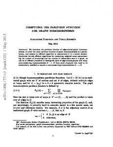
Informally a graph G1 is a minor of another graph G2 (noted G1 4 G2 ) if it can be obtained from it by repeating in some arbitrary order the two following elementary transformations: (a) deleting one edge; (b) contracting one edge, i.e. identifying its two end-vertices into a single vertex and deleting any loop or parallel edges that may arise. We refer to [22] for a more formal definition. In the next two figures, two simple examples of these transformations are shown, which have some relevance in the present context: starting from a planar square lattice, one may form an hexagonal lattice by deleting one edge per site (Figure 1), while the contraction of the same set of edges leads to the triangular lattice (Figure 2).

Figure 1. Example of minor graph obtained by deleting a subset of edges: an hexagonal lattice is formed out of a square lattice.

Figure 2. Example of minor graph obtained by contracting a subset of edges: a triangular lattice is formed out of a square lattice. On the other side, the Pfaffian reduction formula [23] is a well known property of Pfaffians and can be stated as follows.


9

Let A = Aij i,j∈{1,...,2n} a matrix of order 2n and K a subset of the set of indices {1, . . . , 2n}. We denote by AK the sub-matrix of A obtained by deleting all rows and columns not indexed by an element of K. (2.39)

AK = Aij ¯

i,j∈K

Similarly, we denote by AK the antisymmetric matrix indexed by the complementary set of ¯ = {1, . . . , 2n} \ K, which elements are: indices K ¯ ¯ ¯ (2.40) AK ij = − AK ji = Pf A(K∪{i,j}) for all i < j ∈ K

We stress that in definitions (2.39)–(2.40), the order on any subset of indices is the one induced by the order on {1, . . . , 2n}. Pfaffian reduction formula reads:

Proposition 2.41. Let A an antisymmetric matrix of order 2n and K a subset of indices of order 2p, 0 < p < n such that Pf(AK ) 6= 0. We have: −(n−p−1) ¯ (2.42) Pf(A) = Pf(AK ) Pf(AK ) The connection between minor graphs and Pfaffian reduction formula is as follows:

Proposition 2.43. Suppose that G1 = (V1 , E1 ) and G2 = (V2 , E2 ) are two simple graphs such that G1 4 G2 . Consider a transformation which reduces G2 to G1 and denote by E2d (respectively E2c ) the set of deleted (respectively contracted) edges in this transformation. Let AG2 be an incidence matrix (in the sense of 2.22 ) on D(G2 ) such that (2.44)

d 2 AG d1 ,d2 = 0 if either d1 or d2 is incident with an edge in E2

Let K be the set of vertices in D(G2 ) incident with an edge in E2d ∪ E2c . Then the set ¯ ¯ = VD (G2 ) \ K can be identified with VD (G1 ), and the matrix AG2 K defined as in (2.40) K is an incidence matrix on D(G1). In the above proposition, edge contraction (respectively edge deletion) is given a counterpart as a transformation of the incidence matrix associated to the dart graph. Contracting one edge means simply integrating out (using the Pfaffian reduction formula) the corresponding matrix entries. Deleting one edge may have various representations depending on the choice of the reference dimer configuration. Here we take M0 = EDE (G), which is consistent with the general case (proposition 2.18), and edge deletion corresponds to factorizing out the associated edge weight. Note in particular that by Proposition 2.41, both Pfaffians are proportional in some functional sense. Remark 2.45. The minor relation is a partial order on the set of graphs, and in particular the genus of a graph is always larger or equal than the genus of any of its minors. This property does not transfer to the associated dart graphs and D(G1 ) may have a larger genus than D(G2 ) even if G1 4 G2 .

10

THIERRY GOBRON

3. Main results. In this section, we state our main results on the Pfaffian representations of partition functions on a graph G, starting from definitions 2.5 and 2.26. Our first result is the well known theorem due to Kasteleyn [8]. Theorem 3.1. The partition function on a graph G admits a Pfaffian representation if and only if G is planar. The proof presented here is independent on the orientability criterion used by Kasteleyn in his original proof. Instead, we emphasize a connection between this representation problem and McLane’s planarity criterion, Theorem 1.1, which is interesting in its own right. Incidentally, we prove also that in contradistinction with the dimer problem, there is no “Pfaffian” non-planar graph for the Ising model. Furthermore, the approach presented here allows for some new representations of the partition function when G is a non-planar graph. For all positive integer n, let Cn be the multicomplex algebra of order n [29] and Re the linear operator Cn → R which associates to any element its real part. Our main result is the following: Theorem 3.2. Let G = (V, E) be a graph of nonorientable genus g˜. There exist an incidence matrix AG on D(G) (in the sense of 2.22 ) with coefficients in Cg˜, a constant Λ ∈ Cg˜ and a reference perfect matching M0 such that for all edge weight functions on G, the partition function on G can be written as (3.3) ZG (w) = w(M0 ∩ EDE (G)) Re Λ Pf AG,M0 (w) Note that the above expression depend on the non orientable genus [30], that is the minimal number of crosscaps a surface should have to embed G without edge crossings. In the present work, we limit ourselves to the simplest application of Equation (3.3), that is the derivation of an expression of the partition function of a nonplanar graph as a sum of Pfaffians. The first one is in terms of the non orientable genus and involves matrices with complex coefficients:

Corollary 3.4. Let G = (V, E) be a graph of nonorientable genus g˜. There exist a family of incidence matrices (AG j )j∈{1,··· ,2g˜ } on D(G) (in the sense of 2.22 ) with coefficients in C, constants (Λj )j∈{1,··· ,2g˜ } in C and a reference perfect matching M0 such that for all edge weight functions on G, the partition function on G can be written as g ˜

(3.5)

ZG (w) = w(M0 ∩

2 X

EDE (G)) Re

j=1

0 (w) Λj Pf AG,M j

A similar expression has been derived by Tessler [11], building on Kasteleyn’s approach. The nonorientable genus g˜ of a graph G is related to its orientable genus g through the inequality [31] (3.6)

g˜ ≤ 2g + 1

When the graph is non orientably simple (e.g. projective grids), the non-orientable genus can be much smaller than this bound, so that the expansion 3.5 is a real improvement over an expansion in terms of the orientable genus.


11

A proof of inequality (3.6) comes from the fact that starting from any orientable embedding in a surface of genus g, one can construct a nonorientable embedding of nonorientable genus 2g+1. We give an explicit construction on a surface with 2g+1 crosscaps, showing that every edge passes through them an even number of times. As a consequence, both entries of the incidence matrix and constant that appear in Theorem 3.2 can be taken in the subalgebra of C2g+1 generated by even products of generators. This leads to an expansion in terms of 22g Pfaffians of matrices with real coefficients, equivalent to the one stated first by Kasteleyn. Corollary 3.7. Let G = (V, E) be a graph of orientable genus g. There exist a family of incidence matrices (AG j )j∈{1,··· ,4g } on D(G) (in the sense of 2.22 ) with coefficients in R, constants (Λj )j∈{1,··· ,4g } in R and a reference perfect matching M0 such that for all edge weight functions on G, the partition function on G can be written as g

(3.8)

ZG (w) = w(M0 ∩

EDE (G))

4 X

0 Λj Pf AG,M (w) j

j=1

In the rest of the section, we give a sketch of the proof of Theorem 3.1, explain the connection with McLane’s criterion and prepare for the derivation of Theorem 3.2. The first step is built on Proposition 2.43 and is the following Theorem 3.9. Let G1 and G2 be two simple graphs such that G1 4 G2 and AG2 an incidence matrix on D(G2 ). There exists an incidence matrix AG1 on D(G1 ), a constant Λ1,2 and two reference perfect matchings, M1 on D(G1 ) and M2 on D(G2 ), such that for every closed curve C in C(G1 ), (3.10)

FAG1 (M1 , C) = Λ1,2 FAG2 (M2 , Π(C))

where Π : C(G1 ) → C(G2 ) is the canonical mapping induced by the transformation from G2 to its minor G1 . In particular, if the partition function on G2 admits a Pfaffian representation then so does the partition function on G1 . Theorem 3.9 allows here to reduce the class of graphs one has to consider to prove both necessity and sufficiency of the planarity condition. Incidentally, it also clarifies a point raised by Fisher long ago[26], related to the fact that a planar graph has a non planar dart graph if some of its vertices are incident with more than three edges. In such a case, the related dimer problem is no longer solvable and two approaches have been proposed: In Kasteleyn approach [8], one keeps the original graph, and has to argue that the multiplicities encountered are exactly compensated by some sign rule; In Fisher’s approach, one deals with a larger, 3−regular graph so that the dart graph is also planar, and reduces later to the original graph. A consequence of Theorem 3.9 is that both approaches are not only always simultaneously possible, but that Fisher’s planar dimer construction implies Kasteleyn’s sign rule. In the course of the proof of Theorem 3.1, we use Theorem 3.9 twice. On one hand, the proof that planarity is a necessary condition is reduced to an application of Kuratowski’s planarity criterion [27], starting from the following constatation: Proposition 3.11. The partition functions on the complete bipartite graph K3,3 and on the complete graph K5 have no Pfaffian representation.

12

THIERRY GOBRON

On the other hand, Theorem 3.9 and the following lemma allows to arbitrarily restrict the proof of sufficiency to 4-regular graphs, Lemma 3.12. Given a 2-connected simple graph G embedded in some surface S, there exists ˜ embeddable in the same surface such that G 4 G. ˜ a 2-connected 4-regular simple graph G Note that 4-regular graphs are just chosen for convenience. We are left with the following Proposition 3.13. Let G = (V, E) be a 4-regular, 2-connected simple graph with no loops. If G is planar, then its partition function admits a Pfaffian representation. Proof of Proposition 3.13 consists in two parts. First, reduction to 4-regular graphs helps us to write Lemma 2.34 as a set of algebraic equations in the incidence matrix entries, depending on the choice of the cycle basis. We prove next that McLane criterion ( Theorem 1.1 ) is just what is needed to pick a cycle basis so that these algebraic equations do have a consistent solution. First, we introduce some notations. Let G = (V, E) be as in Proposition 3.13. The vertex set of its dart graph D(G) is (3.14) VD (G) = (v, e), v ∈ V, e ∈ E(v)

where E(v) ⊂ E is the set of four edges at vertex v ∈ V . We suppose that the sets V and E(v) for all v ∈ V have been ordered in some arbitrary way and for all v ∈ V we denote by ekv the k th element of E(v). On VD (G), we consider the induced lexicographic order.  ′  v < v (3.15) (v, e) ≤ (v ′ , e′ ) ⇐⇒ or ∀((v, e), (v ′ , e′ )) ∈ VD (G) × VD (G)  v = v ′ and e ≤ e′

Since there is an even number of edge at each vertex, there exists a perfect matching M0 on D(G) such that M0 ∩ E = ∅. Actually there are 3|V | such matchings and we take arbitrarily the following one as our reference perfect matching, [ (3.16) M0 = (v, e1v ), (v, e2v ) , (v, e3v ), (v, e4v ) v∈V

We construct an incidence matrix AG of order |VD (G)| = 4|V |. (3.17)

AG = AG (v,e),(w,f )

(e,f )∈E(v)×E(w) (v,w)∈V ×V

By Definition 2.22, entries of AG are zero except those corresponding to an edge in D(G). If the edge is in EDE (G) (respectively in EDV (G)), e = f (respectively v = w), the coefficent AG (v,e),(w,f ) is termed an “edge entry” (respectively a “site entry”). Recalling that AG is an antisymmetric matrix, we rename all its edge and site entries as follows. For every edge e in E with endvertices v and w such that v < w, we write (3.18)

be = AG (v,e),(w,e)

while for every vertex v ∈ V and every permutation σ on E(v), we define


Sv (σ) = AG (v,σ(e1 )),(v,σ(e2 ))

S¯v (σ) = AG (v,σ(e3 )),(v,σ(e4 ))

AG 3 (v,σ(e1 v )),(v,σ(ev ))

T¯v (σ) = AG (v,σ(e2 )),(v,σ(e4 ))

Uv (σ) = AG (v,σ(e1 )),(v,σ(e4 ))

¯v (σ) = AG 2 U (v,σ(e )),(v,σ(e3 ))

v

(3.19)

13

Tv (σ) =

v

v

v

v

v

v

v

v

v

When σ is the identity, we simplify the notations further as (3.20)

sv = Sv (1) s¯v = S¯v (1)

tv = Tv (1) t¯v = T¯v (1)

uv = Uv (1) u¯v = U¯v (1)

Now let γ = (Vγ , Eγ ) be a cycle of length rγ on G. We consider a cyclic order on both its edge and vertex sets, (3.21) (3.22)

Vγ = (viγ )i∈{1,··· ,rγ } Eγ = (eγi )i∈{1,··· ,rγ }

where the indices are defined modulo rγ so that viγ is incident with eγi−1 and eγi for all i ∈ {1, · · · , rγ }. We want to relate both the order on VD (G) and the order along γ and thus introduce γ-related notations. For all i in {1, · · · , rγ }, we rename the edge entry in AG associated to eγi as, (3.23)

γ Biγ = A(viγ ,eγi ),(vi+1 ,eγi )

Note that Biγ is equal to either +beγi or −beγi according to whether γ goes through edge eγi compatibly or not with the order on VD (G). In order to rename the site entries along γ, we consider the following Lemma 3.24. Let γ a cycle of length rγ ordered as above. For every i ∈ {1, · · · , rγ }, there exists a unique permutation σiγ on E(viγ ) with positive signature such that, eγi−1 = σiγ (e1vγ )

(3.25)

i

eγi

(3.26)

=

σiγ (e4vγ ) i

The effect of the σiγ ’s is to reorder the edges on each site visited by the cycle, so that it enters a site by the first edge and leave by the forth. When considering a given cycle γ, we also simplify notations (3.19) as

(3.27)

Siγ = Sviγ (σiγ ) S¯iγ = S¯viγ (σiγ )

Tiγ = Tviγ (σiγ ) T¯iγ = T¯viγ (σiγ )

Uiγ = Uviγ (σiγ ) ¯vγ (σ γ ) U¯iγ = U i i

The relations between notations (3.20) and (3.27) depend on the actual value of σiγ among twelve possible realizations and are listed in Table 1. Using these notations, we can state the following proposition:

14

THIERRY GOBRON

σiγ (e1v ) σiγ (e2v ) σiγ (e3v ) σiγ (e4v )

Siγ

S¯iγ

Tiγ

T¯iγ

Uiγ

U¯iγ

tv −t¯v

t¯v

uv

u¯v

−tv −t¯v

u¯v −¯ uv

uv −uv

tv

−uv

−¯ uv

e1v

e2v

e3v

e4v

sv

s¯v

e2v e3v

e1v e4v

e4v e1v

e3v e2v

−sv s¯v

−¯ sv sv

e4v

e3v

e2v

e1v

−¯ sv

−sv

−tv t¯v

e1v e3v e4v

e3v e1v e2v

e4v e2v e1v

e2v e4v e3v

tv −tv t¯v

t¯v −t¯v tv

uv −¯ uv −uv

u¯v −uv −¯ uv

sv s¯v −¯ sv

s¯v sv −sv

e2v

e4v

e3v

e1v

−t¯v

−tv

u¯v

uv

−sv

−¯ sv

e1v e4v

e4v e1v

e2v e3v

e3v e2v

uv −uv

u¯v −¯ uv

sv −¯ sv

s¯v −sv

t¯v tv

e2v e3v

e3v e2v

e1v e4v

e4v e1v

u¯v −¯ uv

uv −uv

−sv s¯v

−¯ sv sv

tv t¯v −t¯v −tv

−tv −t¯v

Table 1. Correspondence between the 6 site entries in the upper triangular part of the incidence matrix for a given vertex v (Equation (3.20)), and the new names (Equation (3.27)) after reordering of E(v) = {e1v , e2v , e3v , e4v } according to a cycle γ passing through v (= viγ for some index i). σiγ is the even permutation on E(v) such that γ enters v through edge σiγ (e1v ), and leaves it through σiγ (e4v ) (Lemma 3.24).

Proposition 3.28. Let γ a cycle on G of length rγ and notations as above. If the entries of the incidence matrix AG associated to elements of γ have non zero values and verify the following set of equations: (3.29) Siγ S¯iγ + Tiγ T¯iγ = 0 ∀i ∈ {1, · · · , rγ } γ γ γ ¯γ Ui Ti Ui+1 Ti+1 γ 2 Bi = − γ (3.30) ∀i ∈ {1, · · · , rγ } Si S¯γ i+1

rγ

rγ

(3.31)

Y i=1

Biγ = −

Y

Uiγ

i=1

Then, for any perfect matching M0 such that M0 ∩ E = ∅, the contribution of every closed curve in C(G) is invariant under addition of γ, (3.32)

FAG (M0 , C) = FAG (M0 , C△γ)

∀C ∈ C(G).

Proposition 3.28 will be proven in Section 5, where we introduce a representation in terms of a Grassmann algebra. Equations (3.29)–(3.31) can be obtained by considering all local configurations around γ with an even number of edges at each site. Some of these configurations may not correspond to an actual element C ∈ C(G), for instance when a cut along γ splits the graph G into two pieces, so that some of these equations are possibly not necessary. The set of equations (3.29)–(3.31) always admits a nowhere zero solution, when considering a


15

single cycle. However, compatibility of these conditions for an arbitrary collection of cycles is not granted, even for planar graphs. Here, MacLane’s planarity criterion comes into play as it provides us with a cycle basis B0 with specific properties. In particular, elements of such a basis cannot form a cluster (a double cover of a proper subset of E(v), at some vertex v ∈ V ) [20]. Then the absence of clusters with 3 edges implies compatibility of equations (3.29) for all γ ∈ B0 and all v ∈ V . Similarly, supposing that site entries have been chosen so that equations (3.29) hold for all γ ∈ B0 , the absence of clusters with 2 edges implies that edge entries can be chosen so that equations (3.30) also hold for all γ ∈ B0 . The remaining equations (3.31) are strongly reminding of Kasteleyn’s orientation prescription. Note that equations (3.29)–(3.30) are independent on the sign of the edge entries Biγ , and that once they are solved, one has r r Y Y 2 γ 2 Bi = (3.33) Uiγ i=1

i=1

so that equation (3.31) just amounts to choose independently the sign of the product of edge entries along γ. Existence of a solution to the equations (3.31) for all γ ∈ B0 just derives from independence of the elements in that basis. Proposition 3.28 implies that conditions of Lemma 2.34 are verified for any planar 4-regular graph, and Proposition 3.13 follows. We now generalize these results to non planar graphs. By Theorem 3.1, we already know that a non planar graph G cannot have a cycle basis such that Equations (3.29)–(3.31) can be solved simultaneously for all its elements. The strategy we adopt here consists in finding the largest free family of cycles on which these equations may hold simultaneously and looking at what happens when completing it to a cycle basis. Following the generalization to non planar graphs of McLane’s Theorem [20], we say that a family of cycles on a graph is “sparse” if it contains no cluster, where a cluster is a subfamily of cycles covering twice a proper subset of E(v), for some vertex v. Just as in the planar case, Equations (3.29)–(3.31) can be proven to be simultaneously solvable for all cycles forming a sparse family. Intuitively, a maximal sparse family of cycles has to be related to the embedding properties of the graph, but this relation is rather intricate: in a non planar 2-cell embedding, face boundaries are closed walks but not necessarily cycles and another definition for sparseness is required [20]. The following lemma together with Theorem 3.9 allows us to bypass this point:

Lemma 3.34. Let G1 be a 2-connected simple graph embedded in some surface S. There exists a 4-regular 2-connected graph G2 < G1 embeddable in the same surface S so that all its face boundaries are cycles. If the genus of the embedding in S is minimal for G1 , it is also minimal for G2 since G2 < G1 . When considering such an embedding for G2 in S, the family of face boundaries is a collection of cycles and a sparse family of smallest codimension in C(G2 ). Theorem 3.9 allows then to transfer related results back to G1 4 G2 , even if G1 has no strong embedding of its own genus.

16

THIERRY GOBRON

Hence, we consider a 4-regular graph G = (V, E) with a strong 2-cell embedding in some surface S. We denote by F0 (G) the set of cycles which are face boundaries in that embedding and by F0∗ (G) a maximal free subfamily, obtained by dropping out one element of F0 (G). Clearly F0∗ (G) is a sparse familly and as in the planar case, this property leads to the proof that the algebraic equations (3.29)–(3.30) can be simultaneously solved for all γ ∈ F0∗ (G). A non orientable embedding can be described by an embedding scheme, that is a pair (Π, λ) where Π = (πv )v∈V defines a cyclic ordering of edges at every vertex, and λ : E → {−1, 1} is a signature on the edge set [30]. Note that the correspondence between embeddings and embedding schemes is not one to one, and for a graph with |V | vertices there can be as much as 2|V | embedding schemes describing the same embedding. We prove the following Lemma. Lemma 3.35. Let G a 4-regular graph with a strong 2-cell embedding in some surface S, defined up to homeomorphism by the embedding scheme (Π, λ). There exists an incidence matrix AG with coefficients ( iR if e = f and λ(e) = −1 (3.36) AG for all (v, e), (w, f ) ∈ VD (G) (v,e),(w,f ) ∈ R otherwise. and a reference perfect matching M0 as in (3.16) such that (3.37)

FAG (M0 , C) = FAG (M0 , C△γ)

∀C ∈ C(G), ∀γ ∈ F0∗ (G)

In particular the coefficients of AG can be chosen in R if and only if the embedding is orientable. When the incidence matrix is chosen as in Lemma 3.35, each closed curve C has a weight in the Pfaffian expansion which depends only on its homology class on S. Proof of Theorem 3.2 uses the fact that for a sufficiently large class of graphs, these weights can be easily computed. However, the coefficients have to be chosen in a suitable multicomplex algebra Cn and Lemma 3.35 stated in this larger algebraic context. The more classical expansions (3.5) and (3.8) are then obtained directly by an algebraic reduction from Cn to C and R, respectively. This suggests that expression (3.3) does contain more information than classical expansions, and we believe that it will prove useful to get new results on non planar Ising model. 4. Proofs In this section, we present proofs of all results, with the exception of Propositions 3.28 and 2.41 which are considered in the next section. Proof of Proposition 2.18. If G = (V, E) is the dart graph of some other graph, says G = D(G′ ) and G′ = (V ′ , E ′ ), ′ ′ ′ its edge set is the union of two distinct parts, E = EDV ∪ EDE . Its subgraph (V, EDE ) forms a perfect matching, since by definition, each vertex in V is a dart on G′ and, as such, is ′ incident with exactly one edge of EDE . Proof of Proposition 2.19. Let M be a perfect matching on D(G). For each vertex v ∈ V , denote by E(v) the set of edges at v, and by VD (v) the set of darts at v n (4.1) VD (v) = (v, e), e ∈ E(v)


17

An edge of M is either in EDV and have thus its two endpoints in the same cluster VD (v) for some v ∈ V , or is in EDE and hits two distinct clusters. Since M is a perfect matching on D(G), it hits each of its vertices exactly once. Thus for all v ∈ V , the number of edges in M ∩ EDE which hit VD (v) has the same parity as |VD (v)|. This number, modulo 2 is thus independent on the matching. In particular, if M1 , M2 are two perfect matchings on D(G),we have (4.2)

C = (M1 △M2 ) ∩ EDE = (M1 ∩ EDE )△(M2 ∩ EDE )

and for all v ∈ V , C hits VD (v) an even number of times. Proof of Lemma 2.34 Substituting both Expressions (2.6) and (2.32) in the definition (2.27) and owing to the algebraic independence of the weights, it is clear that the partition function on G admits a Pfaffian representation in the sense of definition 2.26 if and only if there exists an incidence matrix AG a reference perfect matching M0 and a constant Λ 6= 0 such that (4.3)

FAG (M0 , C) = Λ

∀C ∈ C(G)

The actual value of constant Λ is irrelevant , so we only need to verify that for some reference perfect matching, FAG (M0 , ·) is non zero and is equal on any two closed curves in C(G), (4.4)

FAG (M0 , C) = FAG (M0 , C ′ )

for all C, C ′ ∈ C(G)

Now (C(G), △) is a vector space and admits a cycle basis, say BG . Therefore the above set of equations can be reduced to an invariance property under addition of any cycle in that basis (4.5)

FAG (M0 , C) = FAG (M0 , C△γ)

for all C ∈ C(G) and all g ∈ BG

Equations (4.5) are clearly a subset of Equations (4.4); by chain rule, it is easy to show that they generate all of them, so that both sets are equivalent. Proof of Proposition 2.43. Consider two graphs G1 = (V1 , E1 ) and G2 = (V2 , E2 ) such that G1 4 G2 . Consider a given transformation which send G2 on G1 , and denote by E2c (respectively E2d ) the set of contracted (respectively deleted) edges of E2 in that transformation. By construction, each connected component of (V2 , E2c ) is a tree Tv , which is mapped under contraction to a given vertex v in G1 . Furthermore, the edges in E2 \ (E2c ∪ E2d ) are in one to one correspondence with those of E1 , which implies that there is also a one to one correspondence between the set of darts VD (G1 ) and the subset of VD (G2 ) defined as (4.6) K = (v, e) ∈ VD (G2 ), e ∈ E2 \ (E2c ∪ E2d )}

For all d ∈ VD (G1 ), we denote by d˜ its image in K and assume that the order on VD (G1 ) is induced from the order on VD (G2 ) through this correspondence. 2 Let AG2 be an incidence matrix on D(G2 ) such that AG d1 ,d2 = 0 if either d1 or d2 is incident with an edge in E2d ; Then, by (2.40), the matrix [AG2 ]K is an antisymmetric matrix of order |K| = |VD (G1 )|, and for every pair of darts (d1 , d2 ) in VD (G1 ) with d1 < d2 , its entries are (4.7) AdK˜1 ,d˜2 = Pf A(K∪{d˜1 ,d˜2 }

18

THIERRY GOBRON

where (4.8)

K = (v, e) ∈ VD (G2 ), e ∈ E2c ∪ E2d }

In order to prove that AK is an incidence matrix on D(G1 ), we have to check that Equation (2.23) holds for all pairs (d1 , d2 ) ∈ VD (G1 ). Let us consider a pair of darts (d1 , d2 ) such that AdK˜ ,d˜ 6= 0. Then in the expansion of the right hand side of (4.7), there is at least one 1 2 non zero term which necessarily contains as a factor the term Ad˜1 ,d˜2 , or a product of terms Ad˜1 ,˜g1 Ag˜1′ ,˜g2 · · · Ag˜′ ,d˜2 for some k > 0 where (˜ gi , g˜i′ ), 1 ≤ i ≤ k, are pairs of darts associated k to the same edge in E2c (by condition (2.44)). In the first case, Ad˜1 ,d˜2 6= 0 implies (d˜1 , d˜2 ) ∈ ED (G2 ) since A is an antisymmetric incidence matrix. Hence d˜1 and d˜2 contain the same edge in E2 \ (E2c ∩ E2d ), which implies that d1 and d2 also contain the same edge in E1 . In the second case, Ad˜1 ,˜g1 6= 0, Ag˜1′ ,˜g2 6= 0, · · · , Ag˜′ ,d˜2 6= 0 imply that each pair of darts, k d˜1 and g˜1 , g˜1′ and g˜2 , · · · , g˜k′ and d˜2 , share the same vertex, respectively. Since (˜ gi , g˜i′ ) ∈ E2c for all 1 ≤ i ≤ k, these vertices are in the same connected components of (V2 , E2c ) and thus shrink to the same vertex of G1 under contraction. Thus d1 and d2 contain the same vertex in V1 . In both cases, (d1 , d2 ) ∈ ED (G1 ). AK is thus an incidence matrix on D(G1). Proof of Theorem 3.1. Let G be a planar, 2-connected simple graph. By Lemma 3.12, there exists a planar, 2˜ < G, ˜ which partition function admits a Pfaffian representation connected, 4-regular graph G by Proposition 3.13. By Theorem 3.9, this property extends to all its minors and in particular the partition function on G admits a Pfaffian representation. Let G be a non planar graph. Kuratowski’s planarity criterion [27], one of its minors is homeomorphic to the complete graph K5 or the complete bipartite graph K3,3 . By Proposition 3.11, the partition function on either of these two graphs has no Pfaffian representation and by Theorem 3.9, there is also no such Pfaffian representation for the partition function on G. Proof of Theorem 3.2. Let G = (V, E) be a graph of nonorientable genus g˜. We first suppose that G is 4-regular ˜ = (V˜ , E) ˜ with G ˜ 4 G in the following way: we and construct another 4-regular graph G consider a surface S with g˜ crosscaps and decompose it into g˜ + 1 domains D0 , D1 ,· · · ,Dg˜ so that D0 is homeomorphic to a sphere with g˜ holes and each of the Dk , k > 0 is homeomorphic to a Moebius strip. We draw G on S so that all its vertices are in D0 . On every domain Dk , k > 0 , we draw two nested non intersecting simple curves around the crosscap. We ˜ the 4-regular graph which representation on S results from the superposition of the call G representation of G and the 2˜ g closed curves, adding each intersection point to the vertex set , and associating each line segment to an edge. ˜ accordingly so that the all face boundFinally, we possibly use Lemma 3.34 and modify G ˜ ˜ k = (V˜k , E˜k ) the subgraph of aries of G on S are cycles. For every k ∈ {1, · · · , g˜}, we call G ˜ with vertex set the subset of V˜ represented in Dk and edge set the set of edges in E˜ with G both endvertices in V˜k .


19

˜ goes through at most one crosscap. We Note that in this embedding every edge of G ˜ on S so that thus consider an embedding scheme (Π, λ) which describes the embedding of G λ(e) = −1 for every edge e going through a crosscap and λ(e) = +1 otherwise. By Lemma ˜ 3.35, there exists an incidence matrix AG with coefficients as in (3.36), such that equations ˜ (3.29)–(3.31) hold for all cycles γ ∈ F0∗ (G). We introduce a multicomplex algebra Cg˜ with generators i1 , · · · , ig˜ such that i2α = −1 for ˜ all α ∈ {1, · · · , g˜} and iα iβ = iβ iα for all α, β ∈ {1, · · · , g˜}. We construct a new matrix A˜G ˜ with coefficients in Cg˜, so that for every pair of darts (v, e), (w, f ) in VD (G) ( ˜ ˜ k and λ(e) = −1 ik ℑ AG if e = f ∈ G ˜ G (v,e),(w,f ) ˜ A(v,e),(w,f ) = (4.9) ˜ otherwise. AG (v,e),(w,f ) ˜ has its support where ℑ(·) denotes the imaginary part. By construction, every cycle in F0∗ (G) ˜ in one of the subgraphs Gk , or has all edges with +1 signature. ˜ the equations (3.29)–(3.31) contain at most one generator Thus for every cycle γ ∈ F0∗ (G), ˜ ˜ ˜ ik , so that they hold for coefficients of A˜G as soon as they hold for those of AG . Thus A˜G is also an incidence matrix (with coefficients in Cg˜ ) such that equations (3.29)–(3.31) hold for ˜ all cycles γ ∈ F0∗ (G). ˜ has 2g˜ homology classes and any two elements in The set of closed curves on graph G ˜ the same homology class are given the same contribution in the Pfaffian expansion of A˜G . We now construct a particular element in each homology class which contribution can be computed. ˜ ⊂ C(G) ˜ the set of closed curves with support in ∪1≤k≤˜g E˜k . Given Let us denote by CR (G) ˜ the set of perfect a reference perfect matching M0 as in (3.16), we also denote by MR (G) ˜ ˜ matchings in M(G) which have their image in CR (G). (4.10)

˜ = {M ∈ M(G), ˜ ΦM0 (M) ∈ CR (G)} ˜ MR (G)

We also define the following subsets of darts ˜ v ∈ V˜ \ ∪1≤k≤˜g V˜k D0 = (v, e) ∈ VD (G), (4.11) ˜ and for all k ∈ {1, · · · , k} (4.12)

˜ v ∈ V˜k Dk = (v, e) ∈ VD (G),

Obviously the chosen reference perfect matching has its support in ∪0≤k≤˜g Dk × Dk and thus ˜ Now the sets of dimers Dk × Dk , 0 ≤ k ≤ g˜ have also every perfect matching in MR (G). ˜ is a direct product of sets of perfect matchings on each disjoint support, so that MR (G) component. Now define ˜ f0 = FA˜G˜ (M0 , γ0 ) for some γ0 ∈ F0∗ (G) k ˜ k ) \ F ∗ (G) ˜ fk = F ˜G˜ (M0 , γ1 ) for some γ ∈ C(G A

1

0

˜ and C(G ˜ k ) \ F ∗ (G) ˜ is Note that the value of f0 is independent of the choice of γ0 ∈ F0∗(G), 0 k ˜ not empty ( Gk is not planar) and the value of f1 is independent on the choice of γ1 in that set.

20

THIERRY GOBRON

˜ k contains K5 as a minor (which can be formed from the two closed The subgraph G lines around the crosscap and two edges of G passing through the crosscap and their 8 crossing points). Thus by Theorem 3.9, there exists an incidence matrix on K5 which Pfaffian expansion has weights proportional to f0 and fk . In particular they verify Equation (4.62) which is homogeneous. Thus weights f0 and fk verify the same equation, namely, fk f03 = −fk3 f0

(4.13)

Since γ1k passes through the crosscap an odd number of times, fk is necessarily proportional to Ik , which implies then fk = ±ik f0

(4.14)

˜ For conveniency, we possibly change the sign of the coefficients of the matrix A˜G which ˜ equations (3.29)–(3.31) keep are proportional to ik (Indeed, for every cycle γ ∈ F0∗ (G), unchanged in that transformation), so that we can fix those signs to be

(4.15)

fk = ik f0 ˜ Denote by Ck the closed curve in ∈ C(G) ˜ with Now consider a closed curve C ∈ CR (G). ˜ k which coincide with C on G ˜ k and by C0 the null curve. By construction, we support in G have g˜ g˜−1 Y (4.16) FA˜G˜ (M0 , Ck ) = FA˜G˜ (M0 , C) FA˜G˜ (M0 , C0 ) k=1

and thus (4.17)

FA˜G˜ (M0 , C) = f0

g˜ Y

(ik )ǫk

k=1

where (4.18)

( +1 if C|G˜ k has nonorientable genus1 ǫk = 0 otherwise

˜k. where C|G˜ k is the restriction of C on G Setting (4.19) ˜ We get, for every curve C ∈ C(G), (4.20) The Theorem is proven.

g˜ 1 Y Λ= (1 − ik ) f0 k=1

Re ΛFA˜G˜ (M0 , C) = 1

Proof of Corollary 3.4. Let G = (V, E) be a graph of nonorientable genus g˜. By Theorem 3.2, there is an incidence matrix AG on D(G) with coefficients in Cg˜, a constant Λ ∈ Cg˜ and a reference perfect matching M0 such that


(4.21)

21

ZG (w) = w(M0 ∩ EDE (G)) Re Λ Pf AG,M0 (w)

˜ k : Cg˜ → C, k ∈ {1, · · · , 2g˜} such Now there are 2g˜ distincts algebra homomorphisms H ˜ k (ij ) ∈ {−i, +i}, and we have for every element w ∈ C} , that for all j ∈ {1, · · · , g˜}, H g ˜

(4.22)

2 1 X ˜ Re(w) = g˜ Hk (w) 2 k=1

Here we set (4.23)

Λk =

1 ˜ Hk (Λ) 2g˜

and for all (d1 , d2 ) ∈ VD (G) × VD (G) (4.24) and we get

AG k

d1 ,d2

˜ k AG =H d1 ,d2

g ˜

(4.25)

ZG (w) = w(M0 ∩

EDE (G))

2 X

0 Λk Pf AG,M (w) k

k=1

Proof of Corollary 3.7. Let G = (V, E) a graph of orientable genus g. The surface in which it can be minimally embedded can be represented as a (fundamental) polygon with 4g sides to be identified pairwise. Conventionally, the polygon can be represented as a succession of translations along the sides, round the polygon, as (4.26)

−1 −1 −1 −1 −1 Pg = A1 B1 A−1 1 B1 A2 B2 A2 B2 · · · Ag Bg Ag Bg

where A1 , B1 , · · · , Bg−1 are the labels of the sides, and the index −1 indicates an orientation opposite to the previous one. On the other hand, a non orientable surface with genus g˜ can be represented as a fundamental polygon with 2˜ g sides, in the form (4.27)

P˜g˜ = C0 C0 C1 C1 · · · Cg˜−1 Cg˜−1

where each side Ck is followed twice in the same direction. Now we consider (4.26) as an element of the free group F2g generated by the 2g generators A1 , B1 ,· · · , Ag , Bg . and we show hereafter that it can be set in the form (4.27) with g˜ = 2g + 1. We define S0 = T0 = 1F2g and recursively for all 1 ≤ k ≤ g, (4.28)

−1 Sk = Sk−1 Ak Bk A−1 k Bk Tk = Bk Ak Tk−1

22

THIERRY GOBRON

For every 1 ≤ k ≤ g,we write Uk = Sk−1 Ak Bk Tk−1 −1 −1 −1 Vk = Tk−1 Bk−1 A−1 k Sk−1 Tk−1 Bk Tk−1

(4.29)

−1 Wk = Tk−1 Bk−1 Tk−1 Sk−1Tk−1

From these definitions, it follows that , −1 −1 −1 U1 V1 V1 W1 W1 = A−1 (4.30) 1 B1 = T0 A1 B1 and for all k ≥ 2,

−1 −1 −1 Uk Vk Vk Wk Wk Uk−1 Bk−1 Ak−1 Tk−2 A−1 = Tk−1 k Bk

(4.31)

Using these relations, we compute Ug Ug Vg Vg Wg Wg · · · Vk Vk Wk Wk · · · V1 V1 W1 W1 −1 = Sg−1 Ag Bg Tg−1 Ug Vg Vg Wg Wg Ug−1 ··· −1 · · · U1 V1 V1 W1 W1 × · · · Uk Vk Vk Wk Wk Uk−1 −1 −1 −1 = Sg−1 Ag Bg Tg−1 Tg−1 Ag Bg Ag−1 Bg−1 Tg−2 · · · −1 −1 −1 −1 × · · · Tk−1 A−1 k Bk Ak−1 Bk−1 Tk−2 · · · A1 B1 −1 = Sg−1 Ag Bg A−1 g Bg

(4.32)

Which gives the identity Ug Ug Vg Vg Wg Wg · · · Vk Vk Wk Wk · · · V1 V1 W1 W1 −1 −1 −1 = A1 B1 A−1 A2 B2 A−1 · · · Ag Bg A−1 (4.33) 1 B1 2 B2 g Bg

In terms of elements of the free group F2g , we have thus proven an identity between Pg and P˜g˜, with g˜ = 2g + 1, with the following choice for the factors Cj , 0 ≤ j ≤ 2g, (4.34)

C0 = Ug

and for all 0 ≤ k ≤ g − 1, (4.35) (4.36)

C2k+1 = Vg−k C2k+2 = Wg−k

This decomposition proves directly that a graph of orientable genus g can be embedded in a nonorientable surface with 2g + 1 crosscaps and incenditally leads to a proof of inequality (3.6), longer but distinct from the original one [31]. In Figure 3, we give an example of transformation of a fundamental domain for a surface of orientable genus 1 into that of a surface of nonorientable genus 3, according to Identity (4.33). In Figure 4, we show the embedding of a graph of orientable genus 1 in a nonorientable surface with three crosscaps which results from decomposition (4.34)–(4.35), starting from an orientable embedding. Here we are interested in the explicit realization of such a nonorientable embedding. We introduce a multicomplex algebra C2g+1 with generators i0 , i1 , i2g , so that i2k = −1 and ik ik′ = ik′ ik . We now rely on the construction given in the proof of Theorem 3.2. We attach ˜ < G such that an edge generator ik to the crosscap [Ck Ck ]. Considering again a graph G ˜ crosses at most one crosscap, we recall that the edge entries in the incidence matrix AG (v,e),(w,e) are linear in i if and only if edge e crosses the k th crosscap. By Theorem 3.9, the induced k


A B

23

A B

B

B

B A

A

A

B B Figure 3. Left: Fundamental polygon for a surface of genus one, described as a single curve closing at the point marked with a •. Right: transformation of the same curve using decomposition (4.35). The resulting curve now passes three times at the marked point; After identification of these three points, the curve splits into three lobes, each having the structure of a crosscap. incidence matrix for the original graph G gets a similar property: an edge on G corresponds ˜ and its edge entry in AG is proportional to the product of all edge to a simple path in G ˜ entries in AG defined on this path. Accordingly, an edge entry in AG gets a factor ik each times the edge crosses the k th crosscap, and thus is linear in ik if and only if edge e crosses the k th crosscap an odd number of times. Now starting from an orientable embedding of G, we have to read off from expressions (4.34)–(4.35), which crosscaps are crossed oddwise by an edge in G which was originally crossing (once )the boundary of the fundamental domain through side Ak (respectively Bk ), for all 1 ≤ k ≤ g. For this purpose, we have thus to determine for each Cj , 0 ≤ j ≤ 2g, the set of generators O(Cj ) which occur an odd number of times. We have O(C0 ) = Aj , Bj ; 1 ≤ j ≤ g (4.37) and for all k ∈ {0, · · · , g − 1}, Aj , Bj ; 1 ≤ j ≤ g − k − 1 ∪ Ag−k O(C2k+2 ) = Aj , Bj ; 1 ≤ j ≤ g − k − 1 ∪ Bg−k

O(C2k+1 ) =

It is easy to see that each generator appears in an even number of sets. Thus, for any edge crossing the boundary of the fundamental domain, the corresponding edge entry gets proportional to the product of an even number of generators in C2g+1 . Each matrix entry can be thus considered as an element of a subalgebra with generators ek = i0 ik , with ek ek′ = ek′ ek and e2k = 1.

24

THIERRY GOBRON

C1 A C2

C2 BA

B

C0 C0

C1

Figure 4. Left: Embedding on the torus of a graph of orientable genus 1. Right: Derived embedding in a surface with tree crosscaps, with C0 = AB, C1 = B −1 A−1 B, C2 = B −1 . Multiple occurences of the same boundary are identified in two ways: inside each crosscap, opposite boundaries are identified (dashed lines); outside crosscaps, the paired new boundaries are joined by solid lines. By construction, edges do not cross outside crosscaps. Note that every edge goes through a crosscap an even number of times. Simultaneously, the constant Λ defined in Equation (4.19) can be replaced by an element of the subalgebra without changing the real part of Λ Pf(AG,M0 )(w). Namely, we set (4.38)

Λ=

1 f0

X

S⊂{1,··· ,2g} |S|even

(−1)

|S| 2

Y j∈S

ej +

X

S⊂{1,··· ,2g} |S|odd

(−1)

|S|−1 2

Y ej j∈S

We follow the same way as in the proof of Corollary 3.7. We denote by R2g the real ring generated by {ej }1≤j≤2g . There are 22g distincts algebra homomorphisms Hk : R2g → R, k ∈ {1, · · · , 22g } such that for all j ∈ {1, · · · , 2g}, Hk (ej ) ∈ {−1, +1}, and we have for every element w ∈ C} , 2g

(4.39)

2 1 X Re(w) = 2g Hk (w) 2 k=1


25

Here we set 1 Hk (Λ) 2g˜ where Λ is defined by Equation (4.38) and for all (d1 , d2 ) ∈ VD (G) × VD (G) G (4.41) AG k d1 ,d2 = Hk Ad1 ,d2 (4.40)

Λk =

Finally, we get

2g

(4.42)

ZG (w) = w(M0 ∩ EDE (G))

2 X

0 Λk Pf AG,M (w) k

k=1

Proof of Theorem 3.9. We use the same notations as in the proof of Proposition 2.43. We first prove that if G1 4 G2 , there is an isomorphism between C(G1 ) and the subset of closed curves on C(G2 ) not containing deleted edges, ˇ 2 ) = {C ∈ C(G2 ), C ∩ E d = ∅} (4.43) C(G 2

Under contraction, vertices connected through contracted edges are identified to a single vertex, which degree is thus equal modulo 2 to the sum of the degrees of the initial vertices. In particular, closed curves are sent to closed curves, and this allows to define a mapping π0 ˇ 2 ) to C(G1 ), which is surjective by hypothesis since G1 4 G2 . The mapping is also from C(G injective: if two elements in Cˇ have the same image in C(G1 ), they have the same intersection with E2 \ (E2c ∪ E2d ), so that their symmetric difference has its support in E2c and thus vanish, since E2c contains no cycle. This defines a canonical injective mapping Π : C(G1 ) → C(G2 ), such that for all C ∈ C(G1 ), (4.44)

Π(C) = π0−1 (C)

Let AG2 be an incidence matrix on D(G2 ). We first construct a modified incidence matrix AˇG2 as follows. For every pair of darts d1 , d2 in VD (G2 ), let d1 = (v1 , e1 ) and d2 = (v2 , e2 ); we set ( 0 if v1 = v2 and {e1 , e2 } ∩ E2d 6= ∅ G2 ˇ (4.45) Ad1 ,d2 = 2 AG otherwise d1 ,d2 Hereafter we take M2 = EDE (G2 ) ∼ = E2 as the reference perfect matching on D(G2 ) and ˇ consider a closed curve C ∈ C(G2 ). Thus C ∩ E2d = ∅ and Equation (2.20) implies that every ′ perfect matching M in φ−1 M2 (C) contains all pairs of darts {(v, e), (v , e)} in ED (G2 ) such that e ∈ E2d . In particular, AˇG2 and AG2 coincide on every element of M and from Definition (2.33), we get (4.46)

FAˇG2 (M2 , C) = FAG2 (M2 , C)

ˇ 2 ). for all C ∈ C(G ˇ 2 ). By definition, there exists a pair Conversely, consider a closed curve C ∈ C(G2 ) \ C(G ′ ′ ′ of darts d, d in VD (G2 ) with d = (v, e), d = (v , e) and e ∈ C ∩ E2d . Since {d, d′} ∈ M2 , ′ Equation (2.20), implies that for every perfect matching M in φ−1 M2 (C), {d, d } 6∈ M. Hence,

26

THIERRY GOBRON

2 for every such M, there is d′′ = (v, e′′ ) with {d, d′′} ∈ M and by (4.45), AˇG d,d′′ = 0 . The contribution of every perfect matching M in φ−1 M0 (C) is thus zero and

(4.47)

FAˇG2 (M2 , C) = 0

ˇ 2 ). for all C ∈ C(G2 ) \ C(G We now relate the terms in the Pfaffian expansion of AˇG2 to the corresponding terms in the Pfaffian expansion of the incidence matrix on G1 constructed using Proposition 2.43. First, for every weight function w : E1 → R+ , we define its extension w˜ on E2 , as ( w(˜ e) if e ∈ E2 \ (E2c ∪ E2d ) (4.48) w(e) ˜ = 1 if e ∈ E2c ∪ E2d where e˜ is the image in E1 of edge e in E2 \ (E2c ∪ E2d ). ˇ = (Vˇ , E) ˇ be the subgraph of G2 with edge set Eˇ = E c ∪ E d , and vertex set Vˇ the Let G 2 2 ˇ The set of darts on G ˇ is the set K defined set of vertices of G2 incident with some edge in E. ˇ except the null one and in Equation (4.8). By construction there is no closed curve on G d those with a non empty intersection with EE . Since the arguments used to get equations ˇ the nonzero terms in the expansion of Pf [AˇG2 ,M0 (w)] (4.46)–(4.47) apply equally to G, ˜ K are associated to closed curves with no edge in E d . Thus only the set of matchings associated to the null curve contributes, and it has only one element, M2 |Eˇ . More precisely, for every weight function w on E1 , we have (4.49) Pf [AˇG2 ,M0 (w)] ˜ K = ±1 6= 0

which is thus independent on w. The Pfaffian reduction formula 2.41 reads here (n−p−1) ˜ K (4.50) P f [AˇG2 ,M0 (w)] ˜ K = Pf [AˇG2 ,M0 (w)] × Pf(AˇG2 ,M0 (w)) ˜ where 2n = |VD (G2 )| and p = |E2c ∪ E2d |.

By Proposition 2.43 , we already know that [AˇG2 ]K is an incidence matrix on D(G1 ). We claim that the matrix [AˇG2 ,M0 (w)] ˜ K is that the weighted incidence matrix associated to it on D(G1 ) for the weight function w and reference perfect matching M1 = EDE (G1 ) ∼ = E1 . Therefore expanding both sides in equation (4.50), for a generic weight function w on E1 , and identifying terms on both sides using Equation (2.33), one gets F[AˇG2 ]K (M1 , C) = Λ1,2 FAˇG2 (M2 , Π(C)) (4.51)

= Λ1,2 FAG2 (M2 , Π(C))

for all C ∈ C(G1 ), with Λ1,2 = ±1 by Equation (4.49) and Π is the canonical mapping from ˇ 2 ). C(G1 ) onto C(G Suppose now that the partition function on G2 admits a Pfaffian representation. Thus by Lemma 2.34, there exists an incidence matrix AG2 on D(G2 ) such that FAˇG2 (M2 , ·) is ˇ 2 ). By (4.51) and (4.49), F ˇG2 K (M1 , ·) is also constant and different from zero on C(G [A ] constant and different from zero on C(G1 ). Using again Lemma 2.34, this implies that the partition function on G1 also admits a Pfaffian representation. In order to conclude the proof, we have to prove the claim.


27

Given our choice of reference perfect matching, the characterization (2.25) reduces to the identity (4.52)

−1 ˇG2 K [AˇG2 ,M0 (w)] ˜ K d1 ,d2 = w ({d1 , d2 })[A ]d1 ,d2

which has to be checked for every pair of darts d1 , d2 with a common edge in E2 \ (E2c ∪ Ed2 ). ˇ e = (Vˇ ∪{v1 , v2 }, E ˇ ∪{e}) Let d1 = (v1 , e), d2 = (v2 , e) be such a pair of darts. The graph G c ˇ is again a subgraph of G2 , and every closed curve on Ge has either one edge in E2 or has no edge. We have (4.53)

ˇG2 ,M0 (w)] [AˇG2 ,M0 (w)] ˜ K ˜ K∪{d1 ,d2 } ) d1 ,d2 = Pf([A

and the expansion of the Pfaffian on the right hand side thus contains only one term, correˇ e ). In particular,we sponding to the restriction of the reference perfect matching M0 on D(G have Y w˜ −1(e′ ) Pf([AˇG2 ]K∪{d ,d } ) Pf([AˇG2 ,M0 (w)] ˜ K∪{d ,d } ) = 1

1

2

ˇ e′ ∈E

2

e

= w (˜ e) Pf([AˇG2 ]K∪{d1 ,d2 } ) = w −1 (˜ e) [AˇG2 ]K −1

(4.54)

d1 ,d2

Thus Equation (4.52) holds. The theorem is proven.

Proof of Proposition 3.11. Consider first the complete bipartite graph K3,3 . Since it is 3-regular, its dart graph D(K3,3 ) is also 3-regular and there is as many perfect matchings on D(K3,3 ) as there are closed curves on K3,3 . Thus given a reference perfect matching M0 , the mapping φM0 defined in Equation (2.20) is one to one. We label the vertices and edges of K3,3 by letters in {a, b, c, d, e, f } and numbers in {1, · · · , 9}, respectively, as in Figure 5 and if vertex v is incident with edge k, we use the short hand notation vk to denote the dart (v, k). We consider two sets of cycles on K3,3 , S = {γ1 , γ2, γ3 } and S ′ = {γ1′ , γ2′ , γ3′ }, where (4.55)

γ1 = {a, 1, d, 4, b, 6, f, 9, c, 8, e, 2} γ2 = {a, 1, d, 7, c, 9, f, 3} γ3 = {b, 4, d, 7, c, 8, e, 5}

and (4.56)

γ1′ = {a, 1, d, 4, b, 5, e, 8, c, 9, f, 3} γ2′ = {a, 1, d, 7, c, 8, e, 2} γ3′ = {b, 4, d, 7, c, 9, f, 6}

The main property of these two sets is that any subchain of length 4 (a succession of two vertices and two edges in a cycle) appear in both sets with the same multiplicity. For instance the subchain (d, 4, b, 6) appears both in γ1 and γ3′ . Now, drawing simultaneously all cycles in a set on the same surface, slightly shifting each drawing, results in a figure as depicted in Figure 6 with possibly some crossings between the lines of different cycles, and

28

THIERRY GOBRON

d 2

4

1

b

a

6

a2

a1

a3 3

6

7

5

e

f 9

2

8 c

Figure 5. Representation of graph K3,3 in the projective plane (Left) and its dart graph (Right). Vertices and edges are labelled with letters and numbers, as used in text; darts are named accordingly. the number of crossings depends on the surface and the way the cycles are drawn. However, when drawing the two sets S and S ′ on two copies of the same surface, the parity of the number of crossings always differs in both drawings (Figure 6).

Figure 6. The two sets of cycles S (4.55), and S ′ (4.56) are drawn using the representation of K3,3 shown in Figure 5. Both sets have locally the same configurations but parity of the numbers of crossings differ. This property transfers to the perfects matchings on D(K3,3 ) in the following way: We take for instance EDE (K3,3 ) as reference perfect matching, that is, we set (4.57)

M0 = {{a1 , d1}, {a2 , e2 }, {a3 , f3 }, {b4 , d4 }, {b5 , e5 }, {b6 , f6 }, {c7 , d7 }, {c8, e8 }, {c9 , f9 }}


29

so that the two sets of cycles S and S ′ are associated to two sets of perfect matchings, ′ SM = {M1 , M2 , M3 } and SM = {M1′ , M2′ , M3′ }, respectively, where M1 = {{a3 , f3 }, {b5 , e5 }, {c7 , d7 }, {a1 , a2 }, {b4 , b6 }, {c8 , c9 }, {d1 , d4}, {e2 , e8 }, {f6 , f9 }} M2 = {{a2 , e2 }, {b4 , d4 }, {b5 , e5 }, {b6 , f6 }, {c8 , e8 }, {a1 , a3 }, {c7, c8 }, {d1 , d7 }, {f3 , f9 }} M3 = {{a1 , d1}, {a2 , e2 }, {a3 , f3 }, {b6 , f6 }, {c9 , f9 }, {b4 , b5 }, {c7 , c9 }, {d4 , d7}, {e5 , e8 }} and M1′ = {{a2 , e2 }, {b6 , f6 }, {c7 , d7 }, {a1 , a3 }, {b4 , b5 }, {c8 , c9 }, {d1 , d4}, {e5 , e8 }, {f3 , f9 }} M2′ = {{a3 , f3 }, {b4 , d4 }, {b5 , e5 }, {b6 , f6 }, {c9 , f9 }, {a1 , a2 }, {c7 , c8 }, {d1 , d7}, {e2 , e8 }} M3′ = {{a1 , d1}, {a2 , e2 }, {a3 , f3 }, {b5 , e5 }, {c8, e8 }, {b4 , b6 }, {c7, c9 }, {d4 , d7 }, {f6 , f9 }} As a consequence of the properties of sets S and S ′ , here each dimer appears in both sets ′ SM and SM with the same multiplicity. Let A be an arbitrary antisymmetric incidence matrix on D(K3,3 ). The contributions of the cycles in S and S ′ to the Pfaffian expansion of A (equation (2.33) ) are related by (4.58)

3 Y

FA (M0 , γi ) = −

i=1

3 Y

FA (M0 , γi′ )

i=1

This relation derives from the properties of the two sets S and S ′ . It can also be seen also as ′ a property of the perfect matchings in SM and SM alone and any other choice of reference perfect matching would define two equivalent sets of cycles through equation (2.37). Thus for every antisymmetric incidence matrix on D(K3,3 ) and every reference perfect matching there exist two sets of closed curves such that relation (4.58) holds. By Lemma 2.34, the partition function on K3,3 has no Pfaffian representation. The proof for the complete graph K5 is similar. We label the vertices and edges of K5 by letters in {a, b, c, d, e} and numbers in {0, · · · , 9}, respectively, as in Figure 7 and we denote the dart (v, k) by vk . K5 is 4-regular so that the mapping (2.20) is not one to one: in fact K5 has 64 closed curves and D(K5 ) has 416 dimer coverings. We consider two sets of cycles on K5 , S = {γ1 , γ2, γ3 , γ4 } and S ′ = {γ1′ , γ2′ , γ3′ , γ4′ }, where

(4.59)

γ1 γ2 γ3 γ4

= = = =

{a, 4, e, 3, d, 6} {a, 0, b, 1, c, 2, d, 6} {a, 0, b, 7, d, 2, c, 9, e, 4} {a, 0, b, 8, e, 3, d, 2, c, 5}

γ1′ γ2′ γ3′ γ4′

= = = =

{a, 4, e, 9, c, 2, d, 6} {a, 0, b, 8, e, 3, d, 6} {a, 0, b, 7, d, 2, c, 5} {a, 0, b, 1, c, 2, d, 3, e, 4}

and

(4.60)

Here again, any subchain of length 4 (two vertices and two edges) appear in both sets with the same multiplicity. Now, drawing simultaneously all cycles in a set on the same surface, slightly shifting each drawing, results in a figure with some crossings between the

30

THIERRY GOBRON

1 b

0 6

a

8 e

4

5

7

9

d

3

2 c

Figure 7. Representation of graph K5 in the projective plane (Left) and its dart graph in the same representation (Right). Vertices and edges are labelled with letters and numbers, as used in text. lines of different cycles. Again, when drawing the two sets S and S ′ on two copies of the same surface, the parity of the number of crossings always differs in both drawings (Figure 8).

Figure 8. The two sets of cycles S (4.59), and S ′ (4.60) are drawn using the representation of K5 shown in Figure 7. Both sets have locally the same configurations but parity of the numbers of crossings differ. We take EDE (K5 ) as reference perfect matching, that is (4.61)

M0 = {{a0 , b0 }, {b1 , c1 }, {c2 , d2 }, {d3, e3 }, {a4 , e4 }, {a5 , c5 }, {a6 , d6 }, {b7 , d7 }, {b8 , e8 }, {c9 , e9 }}


31

so that each cycle in the two sets S and S ′ are associated to exactly one perfect matchings ′ in SM = {M1 , M2 , M3 , M4 } and SM = {M1′ , M2′ , M3′ , M4′ }, respectively, where M1 M2 M3 M4

= = = =

{{a0 , b0 }, {b1 , c1 }, {c2 , d2 }, {a5 , c5 }, {b7 , d7 }, {b8 , e8 }, {c9 , e9 }, {a4 , a6 }, {d3, d6 }, {e3 , e4 }} {{d3, e3 }, {a4 , e4 }, {a5 , c5 }, {b7 , d7 }, {b8 , e8 }, {c9 , e9 }, {a0 , a6 }, {b0 , b1 }, {c1 , c2 }, {d2, d6 }} {{b1 , c1 }, {d3 , e3 }, {a5 , c5 }, {a6 , d6 }, {b8 , e8 }, {a0 , a4 }, {b0 , b7 }, {c2 , c9 }, {d2, d7 }, {e4 , e9 }} {{b1 , c1 }, {a4 , e4 }, {a6 , d6 }, {b7 , d7 }, {c9, e9 }, {a0 , a5 }, {b0 , b8 }, {c2 , c5 }, {d2, d3 }, {e3 , e8 }}

= = = =

{{a0 , b0 }, {b1 , c1 }, {d3, e3 }, {a5 , c5 }, {b7 , d7 }, {b8 , e8 }, {a4, a6 }, {c2 , c9 }, {d2, d6 }, {e4 , e9 }} {{b1 , c1 }, {c2 , d2 }, {a4 , e4 }, {a5 , c5 }, {b7 , d7}, {c9 , e9 }, {a0 , a6 }, {b0 , b8 }, {d3, d6 }, {e3 , e8 }} {{b1 , c1 }, {d3 , e3 }, {a4 , e4 }, {a6, d6 }, {b8 , e8 }, {c9 , e9 }, {a0 , a5 }, {b0 , b7 }, {c2 , c5 }, {d2, d7 }} {{a5 , c5 }, {a6 , d6 }, {b7 , d7 }, {b8 , e8 }, {c9, e9 }, {a0 , a4 }, {b0 , b1 }, {c1 , c2 }, {d2, d3 }, {e3 , e4 }}

and M1′ M2′ M3′ M4′

As a consequence of the properties of sets S and S ′ , each dimer appears in both sets SM and ′ SM with the same multiplicity. Let A be an arbitrary antisymmetric incidence matrix on D(K5 ). The contributions of the cycles in S and S ′ to the Pfaffian expansion of A (equation (2.33) ) are related by (4.62)

4 Y i=1

FA (M0 , γi ) = −

4 Y

FA (M0 , γi′ )

i=1

This relation derives from the properties of the two sets S and S ′ . It can also be seen also as ′ a property of the perfect matchings in SM and SM alone and any other choice of reference perfect matching would define two equivalent sets of cycles through equation (2.37). Thus for every antisymmetric incidence matrix on D(K5 ) and every reference perfect matching there exist two sets of closed curves such that relation (4.62) holds. By Lemma 2.34, the partition function on K5 has no Pfaffian representation.

Proof of Lemma 3.12. Let G = (V, E) be a finite 2-connected simple graph 2-cell embedded in some smooth sur˜ < G by a succession of elementary transformations face Σ. We construct 4-regular graph G such as vertex splitting, edge addition and edge subdivision [30], taking care that at each step, the resulting graph is still a 2-connected simple graph embeddable in the same surface. We first state the following three claims, which we prove for any 2-connected simple graph G 2-cell embedded in some smooth surface Σ: • Claim 1: If some vertex in graph G has odd valency, there exists a 2-connected simple graph G′ < Gembeddable in the same surface, with a strictly smaller number of vertices of odd valency. • Claim 2: If all vertices in G have even valency and some vertex in G has valency larger than 4, there exists a 2-connected simple graph G′ < G embeddable in the same surface, with all vertices of even valency and a strictly smaller number of vertices of valency larger than 4.

32

THIERRY GOBRON

• Claim 3: If some vertex in G has valency 2 and all others of valency 4, there exists a 2-connected simple graph G′ < Gembeddable in the same surface, with a strictly smaller number of vertices of valency 2, and all others of valency 4. Clearly, the proof of Lemma 3.12 follows easily from the above three claims and transitivity of · < · : a finite iteration of Claim 1 leads to a graph G′ < G with all vertices of even valency. Claim 2 allows then for the construction of a graph G′′ < G′ with all vertices of valency 2 or 4. Finally a repeated use of Claim 3 gives a 4-regular graph G′′′ < G′′ . We now prove the above three claims. Proof of Claim 1. Suppose that G is a 2-connected simple graph 2-cell embedded in some smooth surface Σ and that some vertex has odd valency. Since the number of such vertices is necessarily even, one can pick a pair of them, says v1 , v2 . If they belong to the same face boundary, we construct a graph G′ by adding an edge {v1 , v2 } (or a new vertex v and two edges {v1 , v}, {v, v2 } if v1 and v2 are adjacent on G). If v1 , v2 don’t belong to the same face boundary, one considers a finite sequence of faces {Fj }j=0,k such that v1 ∈ F 0 , v2 ∈ F k and the boundaries of Fj−1 and Fj share at least one edge, says ej , for all 1 < j ≤ k. We chose this sequence to be of minimal length and construct G′ by replacing each edge ej by a new vertex wj and two new edges, each with endvertices wj and a distinct endvertex of ej (namely, subdividing each edge ej ), and adding k +1 edges {v1 , w1 }, {w1 , w2 },· · · ,{wk , v2 }. In both cases, v1 and v2 have even valency in G′ , while all new vertices have valency 2 or 4. In addition G′ is a 2-connected simple graph since G is and the endvertices of new edges are not neighbors in G. Finally G′ can be embedded in the same surface Σ since the transformation consists in splitting one or more faces of the embedding of G. Proof of Claim 2. Suppose now that all vertices of G have even valency and let v a vertex of valency r > 4. We construct a new graph G′ by replacing this vertex in G and its r edges by a 4-regular tree Tv with r−2 points, r external edges and r−4 internal edges. Since 2 2 a sufficiently small neighborhood of xv is homeomorphic to a disk and Tv of genus zero, one can identify the external edges of this tree with the edges of v in G in such a way that G′ can still be embedded on Σ. By construction G′ is still a simple graph and it is 2-connected since no new vertex is separating. Proof of Claim 3. Suppose that some vertices of G have valency 2 and all others valency 4. Let v be a vertex of valency 2. If G is a simple graph distinct from K3 , one of the faces of the embedding which contains v has length at least 4, so one can pick two distinct edges on the boundary of this face with endvertices distinct from v. Now one construct G′ from G by adding one subdivision vertex on these two edges , says w1 and w2 and the three edges {v, w1}, {v, w2 } and {w1 , w2 }. the three points v, w1 and w2 have valency 4 in G′ so G′ has one point of valency 2 less than G. Furthermore the transformation consists in splitting a face so that G′ can still be embedded in Σ. Furthermore G′ is again a 2-connected simple graph. If G identifies to the graph K3 , one may consider K2,2 < K3 , and proceed as above.

Proof of Proposition 3.13. Let G = (V, E) be a planar 2-connected 4-regular graph and BG a cycle basis on G as in McLane’s planarity criterion 1.1. An important property of such a basis is that none of its subsets can form a double cover of a proper subset of E(v), for any vertex v ∈ V . For completeness, we give here a short proof of this property [20]:


33

Suppose that this property is false at some vertex v, and call a cluster the proper subset of E(v) covered twice. Since BG verifies McLane’s criterion, every element of BG either belong to the covering and has two edges in the cluster, or does not belong to it, and has thus 0 edges in it. The intersection with the cluster thus contains an even number of edges and this holds true also for all elements generated from BG by finite difference. However, by hypothesis, there is at least one edge at v outside the cluster, and since G is 2-connected, there exists a cycle in C(G) containing whichever pair of edges in E(v); and in particular exactly that edge and one edge in the cluster. This is in contradiction with the fact that BG is a cycle basis for C(G), which proves the above property. We now consider an incidence matrix AG and notations as in (3.18)–(3.27). We prove that conditions of Proposition 3.28 can hold simultaneously for all cycles in BG . We first consider the site equations (3.29). Let v ∈ V and γ ∈ BG such that γ ∋ v. When rewritten in the original variables (see Table 1), the related site equation may appear in three different forms, depending on which edges in E(v) belong to γ:

(4.63)

sv s¯v + tv t¯v = 0 tv t¯v + uv u¯v = 0 uv u¯v + sv s¯v = 0

if γ ∩ E(v) = {e1 , e4 } or {e2 , e3 } if γ ∩ E(v) = {e1 , e2 } or {e3 , e4 } if γ ∩ E(v) = {e1 , e3 } or {e2 , e4 }

Equations at different vertices are obviously independent. Suppose that there are two cycles in BG passing through v and associated to a different equation in (4.63). They share necessarily exactly one edge in E(v). Now take any other cycle in BG passing through v. By McLane’s criterion, it can neither share the common edge (already appearing twice), nor share a distinct edge with each (which would form a cluster of 3). Thus it is necessarily disjoint in E(v) from one of the other cycle, and the associated equation is the same. Thus at every vertex v, the site equations associated to all elements of BG are at most two, and admit a nowhere zero solution. Note that all three equations together have no nowhere zero solution as it would give sv s¯v = tv t¯v = uv u¯v = 0. We suppose from now on that site entries of the incidence matrix have been given non zero values so that all site equations hold for all γ ∈ BG , and we consider the set of edge equations. We consider a cycle γ = (Vγ , Eγ ) in BG with its elements ordered as in Equations (3.21)– (3.22). For every pair (v, e) ∈ Vγ × Eγ with v incident on e, we define the following ratio  γ γ U T¯   if ∃ i ∈ {1, · · · , rγ } such that e = eγi and v = viγ  i γi S γ = Uγi T γ (4.64) Rv,e  γ i+1 i+1  if ∃ i ∈ {1, · · · , rγ } such that e = eγi and v = vi+1  ¯Γ Si+1

γ The ratio Rv,e depends on the intersection of γ with E(v), and is independent on its orientation. On each vertex, this ratio may take twelve different expressions in terms of the edge entries, which can be computed from Table 1 and are reported here in Table 2.

34

THIERRY GOBRON ′ e e

e1v

e1v

e2v

e3v

e4v

sv u v t¯v

tv sv u¯v

uv tv s¯v

u¯v t¯v s¯v

t¯v sv uv

e2v

sv u¯v tv

e3v

tv s¯v uv

u¯v tv sv

e4v

uv t¯v sv

t¯v s¯v u¯v

s¯v u¯v t¯v s¯v uv tv

γ Table 2. Expression of the ratio Rv,e for a vertex v, an edge e and a cycle γ such that γ ∩ E(v) = {e, e′ }. This expression is written as a function of the location of e, e′ in the ordered set E(v) = {e1v , e2v , e3v , e4v }.

Let e be an edge on graph G with endvertices v and w, and γ be a cycle in BG containing e. The associated edge equation reads (4.65)

γ γ b2e = −Rv,e Rw,e

Now consider two distinct cycles γ and γ ′ in BG passing through a same edge e with endvertex v. By McLane’s criterion, they cannot have two successive edges in common, since it would form a cluster of two edges. Thus, up to a permutation, and possibly, exchanging the roles of γ and γ ′ , one can suppose that γ ∩ E(v) = {e1v , e4v } and γ ′ ∩ E(v) = {e1v , e2v }, so that e1v is their common edge at v. From Table 2, the associated ratios read uv tv γ Rv,e 1 = v s¯v sv u v γ′ Rv,e1v = t¯v The site equation associated to γ at v reads sv s¯v + tv t¯v = 0 which implies ′

γ γ Rv,e 1 = −Rv,e1 v v

This relation is invariant under any even permutation on E(v), so we get the following result. Two distinct cycles γ and γ ′ in BG passing through a same edge e with endvertex v have opposite ratio: (4.66)

′

γ γ Rv,e = −Rv,e

Thus, since the left hand side of Equation (4.65) is quadratic in the ratios,it is invariant when considering different cycles in BG passing through the same edge. Thus edge equations are identical for different cycles at the same edge, and are also algebraically independent for different edges. Hence, the whole set of edge equation can be solved simultaneously for all edges and all cycles in BG .


35

We now assume that the coefficients of the incidence matrix have been chosen so that both site and edge equations are fulfilled, and consider the cycle equations (3.31), for all cycles in BG . We first note that these equations are not fully independent from the edge and site equations. Multiplying all edge equations associated to a given cycle γ ∈ BG gives rγ rγ rγ γ ¯γ ¯ γ 2 Y Y Y 2 T T U i i i γ 2 rγ Bi = (−1) (4.67) U¯iγ = γ ¯γ S S i=1

i=1

i

i

i=1

where the last equality comes from the use of site equations (3.29). Thus for every cycle γ ∈ BG , we have rγ rγ Y Y γ U¯iγ Bi = −ǫγ (4.68) i=1

i=1

with ǫγ ∈ {−1, 1}. We thus define a new set of variables {ǫe }e∈E with value in {−1, 1}, and consider the set of equations (4.69)

Y

ǫe = ǫγ

e∈γ

for all γ in BG . Now the independence of the cycles as elements of the (vector) basis BG implies the independence of equations in (4.69) and thus insures the existence of a solution with {ǫe }e∈E in {−1, 1}. Now for every edge e such that ǫe = −1, we change the sign of the two associated edge entries in the incidence matrix. The new edge and site entries are all nonzero and such that Equations (3.29)–(3.31) hold for all cycles in BG . Thus, by Proposition 3.28, there exists a reference perfect matching M0 such that Equation (3.32) holds for all cycle γ ∈ BG . By Lemma 2.34, the partition function on G admits a Pfaffian representation.

Proof of Lemma 3.24. For every vertex v, the set of permutations on E(v) is homeomorphic to S4 . There are exactly two permutations σ in S4 , with a prescribed value of two images, which differ by a transposition. Thus they have a different signature and only one has a positive one. The twelve permutations are listed explicitely in the first column of Table 1. Proof of Lemma 3.34. Suppose G1 is a 2-regular simple graph embedded in some surface S. Using Lemma 3.12, there exists a 4-regular, 2-connected simple graph G′0 < G1 embedded in the same surface. Let K be the number of faces in this embedding which closure is not homeomorphic to a closed disk. If k 6= 0, we construct recursively a sequence of graphs G′1 , . . . , GK such that G′k < G′k−1 for all k ∈ {1, · · · , K} so that G′K has a strong embedding in S. For k in {0, · · · , K − 1}, suppose that G′k is embedded in S . We pick one face which closure is not homeomorphic to a closed disk, and denote by γ the closed path around this face, which can be described as a succession of vertices and edges as (4.70)

γ = {v1 , e1 , · · · , vi , ei , · · · , vr , er }

36

THIERRY GOBRON

where r is the length of the path and {vi }i∈{1,··· ,r} (respectively {ei }i∈{1,··· ,r} ) are vertices (respectively edges) in G′k such that vi is incident with ei−1 and ei for all i ∈ {1, · · · , r} (we assume that indices are defined modulo r). Since γ is a path round a face, every edge in γ appears at most twice and successive edges have to be distinct (since G′k has no vertex incident with only one edge). Denote by I1 ⊂ {1, · · · , r} the indices of edges appearing only once in γ and by I2 the set of pairs of indices associated to edges appearing twice in γ (4.71)

I2 = {(i, j), 1 ≤ i < j ≤ r, ei = ej }

We construct Gk′ +1 starting from G′k as follows: on each edge on the path, we add one (respectively two) subdivision points according to its number of occurrences in γ. In other words, we add r vertices {wi }i∈{1,··· ,r} to G′k , delete all edges in γ and replace ei by two edges (vi , wi ) and (wi , vi+1 ) if i ∈ I1 , or by three edges (vi , wi ) (wi , wj ) and (wj , vi+1 ) if (i, j) ∈ I2 . Finally we add r edges between subdivision points, (w1 , w2 ), (w2 , w3 ), . . . , (wr , w1 ). Note that each new edge has its endvertices on successive edges on the boundary of the face, they can be drawn on it without crossing, so that the resulting graph G′k+1 can be embedded on the same surface S. Furthermore, it is 4-regular, since new vertices have four edges incident on it, and 2-connected since G′k is. Gk′ +1 has r more vertices and 2r more edges than Gk . On the embedding on S, the r + 1 new faces have length 3, 4, 5 or r, and are all bounded by cycles since all their vertices are distinct. Other faces have not changed except by possibly adding one subdivision point on some edges, and there is one face less which boundary is not a cycle. Finally Gk′ +1 < Gk since it is constructed from it by adding subdivision points and edges. Thus, starting from G′0 and iterating K times this construction, we obtain a graph G′K embedded in S with all faces bounded by cycles. Graph G′K is 4-regular and 2-connected and by transitivity, we also have G′K < G1

Proof of Lemma 3.35. The proof of this lemma is partly similar to that of Proposition 3.13. In fact, as in the planar case, no subset of F0∗ (G) can form a cluster, that is a double cover of a proper subset of E(v)) at some vertex v ∈ V . This implies that all results in the proof of Proposition 3.13 hold true in the non planar orientable case, for the restricted set of cycles F0∗ which generates the face system and not for the whole basis. For every v in V , the associated vertex equations consist in a system of two equations out of the three possible ones written in Equation (4.63), which has clearly solutions in R. Therefore we suppose from now on that all vertex entries of the incidence matrix have been given a real non zero value so that the set of vertex equations for all vertices and all cycles in F0∗ (G), are fulfilled. γ We now consider the ratios Rv,e defined in 4.64. We have already noted that their value does not depend on the orientation of the associated cycle γ, and that if two cycles pass trough the same edge, the ratios have opposite value. Here we show that the two ratios associated to the same cycle γ at a given vertex, says viγ , have values with opposite signs.


37

Indeed, from the definition (4.64), we have Rvγγ ,eγ i i

(4.72)

Rvγγ ,eγ

(4.73)

i

i−1

Uiγ T¯iγ = Siγ UγT γ = i¯γ i Si

while the vertex equation reads Siγ S¯iγ + Tiγ T¯iγ = 0

(4.74) and thus (4.75)

Rvγγ ,eγ Rvγγ ,eγ i

i

i

i−1

= − Uiγ

2

γ 0 and Rv,πv (e) < 0 for all edges e ∈ E(v) and all cycles γ such that γ ∩ E(v) = {e, πv (e)}, or all signs are simultaneously reversed. We also note that given a solution (sv , tv , uv , s¯v , t¯v , u¯v ), one gets another solution by reversing the signs of uv and u¯v , for which all ratio at v change sign. Thus given a rotation system Π = (πv )v∈V , one can choose the solutions of the site γ equations so that the ratios Rv,e > 0 simultaneously for all v ∈ V , all e ∈ E(v) and all ∗ γ ∈ F0 (G) such that γ ∩ E(v) = {e, πv (e)}. Now consider an edge e ∈ E with endvertices v and w. If its signature λ(e) = +1, a cycle γ passing through e behaves either according to πv on v and πw on w, or according to πv−1 on v and πw−1 on w. Thus either γ ∩ E(v) = {πv−1 (e), e} and γ ∩ E(w) = {e, πw (e)}, or γ γ γ ∩ E(w) = {πw−1 (e), e} and γ ∩ E(v) = {e, πv (e)}. Therefore the two ratios Rv,e and Rw,e have opposite sign and the associated edge equation

(4.76)

γ γ b2e = −Rv,e Rw,e >0

has a solution in R. In the other case, λ(e) = −1, a cycle γ passing through e behaves either according to πv on v and πw−1 on w, or according to πv−1 on v and πw on w. Thus either γ ∩ E(v) = {πv−1 (e), e} and γ ∩ E(w) = {πw−1 (e), e} , or γ ∩ E(w) = {e, πw (e)} and γ γ γ ∩ E(v) = {e, πv (e)}. In that case, the two ratios Rv,e and Rw,e have the same sign and the associated edge equation (4.77)

γ γ b2e = −Rv,e Rw,e